example_likert

In [1]:

import arviz as az
import matplotlib.pyplot as plt
import numpy as np
import pandas as pd
import pymc as pm
import pytensor.tensor as pt
import statsmodels.api as sm

from scipy.stats import bernoulli
from statsmodels.miscmodels.ordinal_model import OrderedModel

WARNING (pytensor.tensor.blas): Using NumPy C-API based implementation for BLAS functions.

In [2]:

plt.rcParams["font.family"] = "Latin Modern Roman"

In [3]:

%config InlineBackend.figure_format = 'retina'  # high resolution figures
az.style.use("arviz-darkgrid")
rng = np.random.default_rng(42)

In [4]:

def make_data():
    np.random.seed(100)
    salary = np.random.normal(40, 10, 500)
    work_sat = np.random.beta(1, 0.4, 500)
    work_from_home = bernoulli.rvs(0.7, size=500)
    work_from_home_calc = np.where(work_from_home, 1.4 * work_from_home, work_from_home)
    latent_rating = (
        0.08423 * salary
        + 0.2 * work_sat
        + work_from_home_calc
        + np.random.normal(0, 1, 500)
    )
    explicit_rating = np.round(latent_rating, 0)
    df = pd.DataFrame(
        {
            "salary": salary,
            "work_sat": work_sat,
            "work_from_home": work_from_home,
            "latent_rating": latent_rating,
            "explicit_rating": explicit_rating,
        }
    )
    return df


try:
    df = pd.read_csv("../data/fake_employee_manger_rating.csv")
    df = df[
        ["salary", "work_sat", "work_from_home", "latent_rating", "explicit_rating"]
    ]
except FileNotFoundError:
    df = make_data()

K = len(df["explicit_rating"].unique())
df.head()

	salary	work_sat	work_from_home	latent_rating	explicit_rating
0	22.502345	0.735425	1	1.376997	1.0
1	43.426804	0.570354	0	5.419863	5.0
2	51.530358	0.738212	0	5.279701	5.0
3	37.475640	0.346045	1	4.651830	5.0
4	49.813208	0.365451	1	5.788661	6.0

In [5]:

fig, axs = plt.subplots(1, 3, figsize=(15, 5))
axs = axs.flatten()
ax = axs[0]
ax.scatter(
    df["salary"],
    df["explicit_rating"],
    label="Explicit Rating",
    color="navy",
    alpha=0.3,
)
axs[1].scatter(
    df["work_from_home"],
    df["latent_rating"],
    label="Latent Rating",
    color="maroon",
    alpha=0.3,
)
axs[1].scatter(
    df["work_from_home"],
    df["explicit_rating"],
    label="Explicit Rating",
    c="navy",
    alpha=0.3,
)
axs[2].scatter(
    df["work_sat"], df["latent_rating"], label="Latent Rating", color="maroon", alpha=0.3
)
axs[2].scatter(
    df["work_sat"],
    df["explicit_rating"],
    label="Explicit Rating",
    color="navy",
    alpha=0.3,
)
ax.scatter(df["salary"], df["latent_rating"], label="Latent Sentiment", color="maroon")
ax.set_title("Manager Ratings by Salary")
axs[1].set_title("Manager Ratings by WFH")
axs[2].set_title("Manager Ratings by Work Satisfaction")
ax.set_ylabel("Latent Sentiment")
ax.set_xlabel("Employee Salary")
axs[1].set_xlabel("Work From Home: Y/N")
axs[2].set_xlabel("Employee Work Satisfaction")
axs[1].legend()

plt.show()

In [6]:

exog = sm.add_constant(df[["salary", "work_from_home", "work_sat"]])
mod = sm.OLS(df["explicit_rating"], exog)
results = mod.fit()
results.summary()

results.predict([1, 200, 1, 0.6])
fig, axs = plt.subplots(1, 2, figsize=(20, 6))
axs = axs.flatten()
ax = axs[1]
salaries = np.linspace(10, 125, 20)
predictions = [results.predict([1, i, 1, 0.6])[0] for i in salaries]
ax.plot(salaries, predictions, label="Implied Linear function of Salaries on Outcome")
ax.set_title("Out of bound Prediction based on Salary")
ax.axhline(10, linestyle="--", color="black")
ax.set_xlabel("Hypothetical Salary")
ax.set_ylabel("Manager Rating Scale")
ax.axhline(0, linestyle="--", color="black")
axs[0].hist(results.resid, ec="white")
axs[0].set_title("Simple OLS Residuals on Training Data")

Text(0.5, 1.0, 'Simple OLS Residuals on Training Data')

In [7]:

def constrainedUniform(N, min=0, max=1):
    return pm.Deterministic(
        "cutpoints",
        pt.concatenate(
            [
                np.ones(1) * min,
                pt.extra_ops.cumsum(pm.Dirichlet("cuts_unknown", a=np.ones(N - 2))) * (max - min)
                + min,
            ]
        ),
    )

In [8]:

def make_model(priors, model_spec=1, constrained_uniform=False, logit=True):
    with pm.Model() as model:
        if constrained_uniform:
            cutpoints = constrainedUniform(K, 0, K)
        else:
            sigma = pm.Exponential("sigma", priors["sigma"])
            cutpoints = pm.Normal(
                "cutpoints",
                mu=priors["mu"],
                sigma=sigma,
                transform=pm.distributions.transforms.ordered,
            )

        if model_spec == 1:
            beta = pm.Normal("beta", priors["beta"][0], priors["beta"][1], size=1)
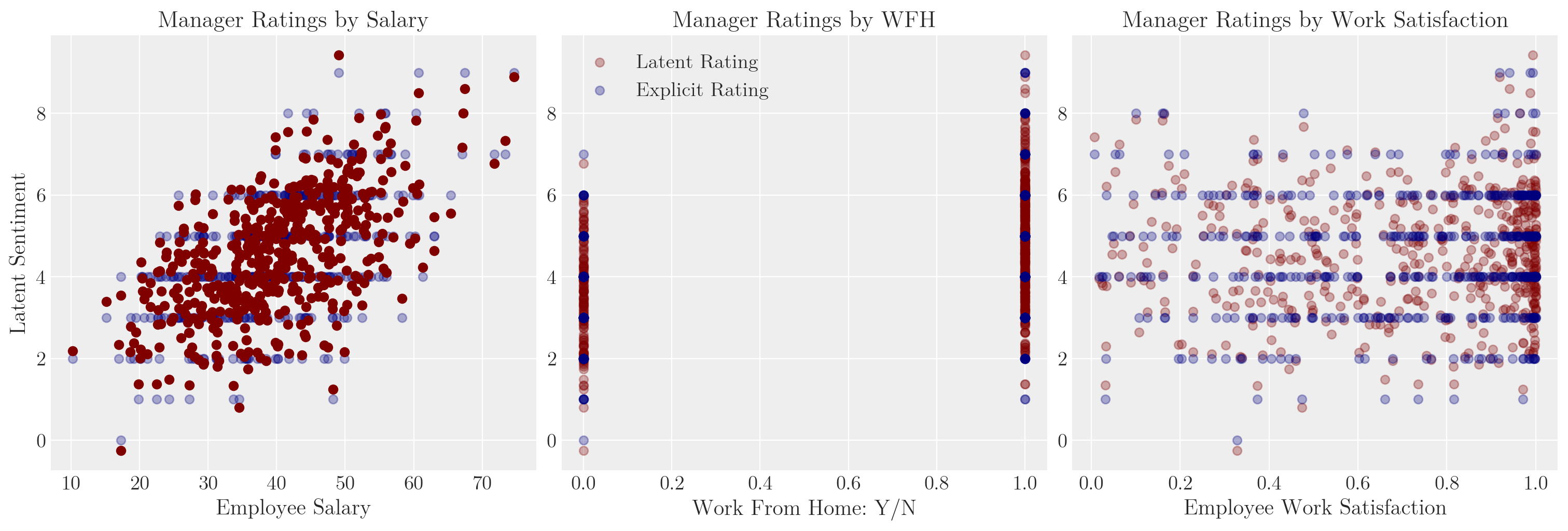
            mu = pm.Deterministic("mu", beta[0] * df.salary)
        elif model_spec == 2:
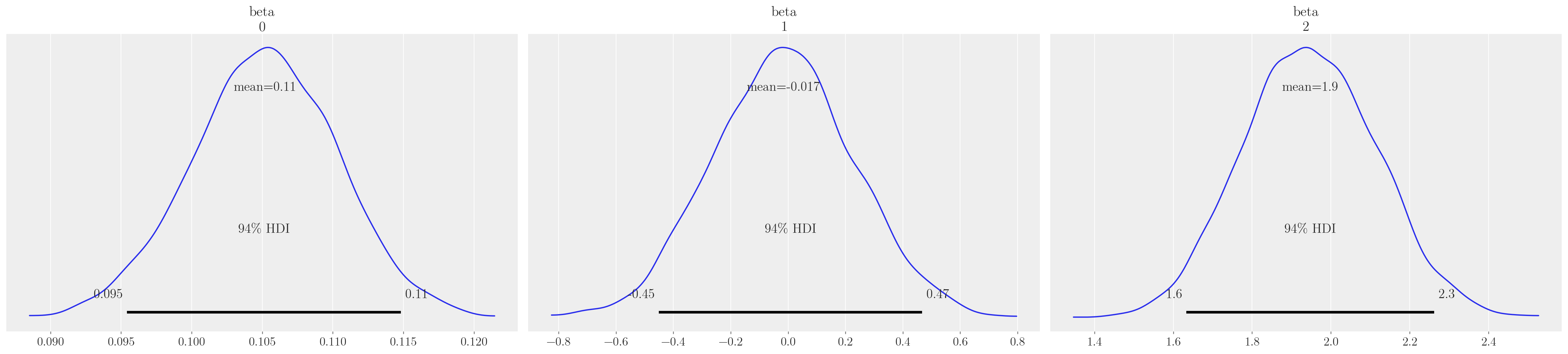
            beta = pm.Normal("beta", priors["beta"][0], priors["beta"][1], size=2)
            mu = pm.Deterministic("mu", beta[0] * df.salary + beta[1] * df.work_sat)
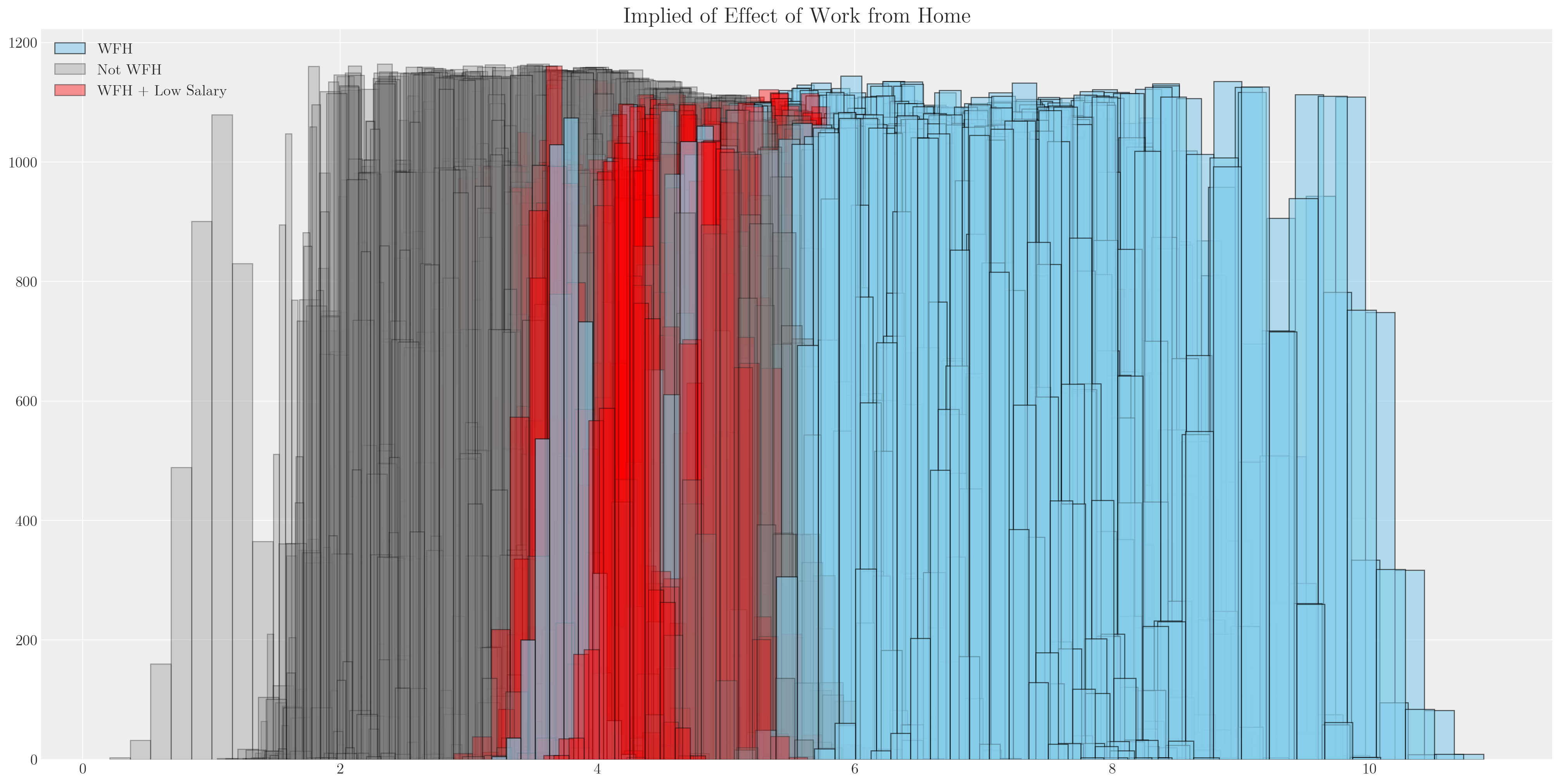
        elif model_spec == 3:
            beta = pm.Normal("beta", priors["beta"][0], priors["beta"][1], size=3)
            mu = pm.Deterministic(
                "mu", beta[0] * df.salary + beta[1] * df.work_sat + beta[2] * df.work_from_home
            )
        if logit:
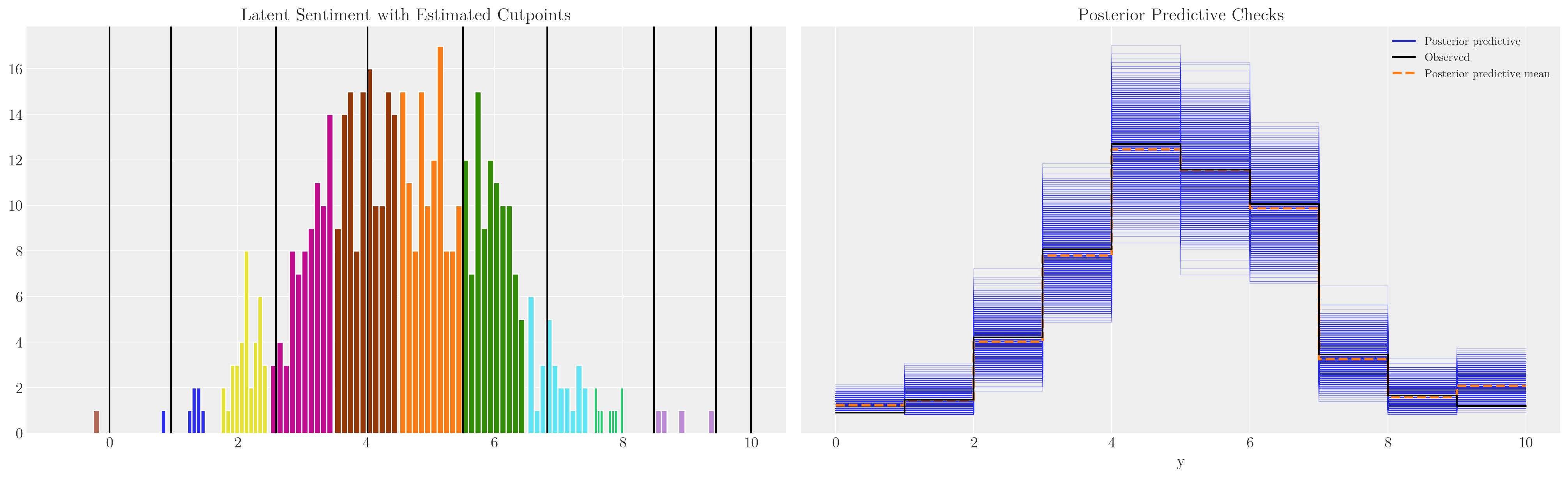
            y_ = pm.OrderedLogistic("y", cutpoints=cutpoints, eta=mu, observed=df.explicit_rating)
        else:
            y_ = pm.OrderedProbit("y", cutpoints=cutpoints, eta=mu, observed=df.explicit_rating)
        idata = pm.sample(nuts_sampler="numpyro", idata_kwargs={"log_likelihood": True})
        idata.extend(pm.sample_posterior_predictive(idata))
    return idata, model


priors = {"sigma": 1, "beta": [0, 1], "mu": np.linspace(0, K, K - 1)}
idata1, model1 = make_model(priors, model_spec=1)
idata2, model2 = make_model(priors, model_spec=2)
idata3, model3 = make_model(priors, model_spec=3)
idata4, model4 = make_model(priors, model_spec=3, constrained_uniform=True)
idata5, model5 = make_model(priors, model_spec=3, constrained_uniform=True)

There were 86 divergences after tuning. Increase `target_accept` or reparameterize.
The rhat statistic is larger than 1.01 for some parameters. This indicates problems during sampling. See https://arxiv.org/abs/1903.08008 for details
The effective sample size per chain is smaller than 100 for some parameters.  A higher number is needed for reliable rhat and ess computation. See https://arxiv.org/abs/1903.08008 for details
Sampling: [y]

There were 83 divergences after tuning. Increase `target_accept` or reparameterize.
The rhat statistic is larger than 1.01 for some parameters. This indicates problems during sampling. See https://arxiv.org/abs/1903.08008 for details
Sampling: [y]

There were 1 divergences after tuning. Increase `target_accept` or reparameterize.
Sampling: [y]

Sampling: [y]

Sampling: [y]

In [9]:

az.summary(idata3, var_names=["sigma", "cutpoints", "beta"])

	mean	sd	hdi_3%	hdi_97%	mcse_mean	mcse_sd	ess_bulk	ess_tail	r_hat
sigma	2.237	0.733	0.845	3.551	0.017	0.012	1752.0	1723.0	1.0
cutpoints[0]	-0.741	0.962	-2.649	0.953	0.023	0.017	1774.0	2082.0	1.0
cutpoints[1]	1.728	0.559	0.666	2.747	0.011	0.008	2457.0	2800.0	1.0
cutpoints[2]	3.801	0.527	2.842	4.813	0.012	0.009	1859.0	1882.0	1.0
cutpoints[3]	5.395	0.549	4.324	6.394	0.013	0.009	1716.0	1772.0	1.0
cutpoints[4]	7.047	0.602	5.891	8.185	0.015	0.010	1643.0	1705.0	1.0
cutpoints[5]	8.511	0.651	7.309	9.781	0.016	0.012	1598.0	1729.0	1.0
cutpoints[6]	10.475	0.725	9.054	11.783	0.018	0.013	1574.0	1692.0	1.0
cutpoints[7]	11.889	0.802	10.385	13.388	0.020	0.014	1614.0	1533.0	1.0
cutpoints[8]	13.237	0.939	11.543	15.113	0.023	0.016	1727.0	1741.0	1.0
beta[0]	0.133	0.011	0.113	0.154	0.000	0.000	1886.0	2062.0	1.0
beta[1]	0.211	0.278	-0.294	0.734	0.004	0.004	4208.0	3087.0	1.0
beta[2]	2.319	0.216	1.907	2.712	0.004	0.003	2496.0	2988.0	1.0

In [10]:

pm.model_to_graphviz(model3)

In [11]:

implied_probs = az.extract(idata3, var_names=["y_probs"])
implied_probs.shape

(500, 10, 4000)

In [12]:

implied_probs[0].mean(axis=1)

<xarray.DataArray 'y_probs' (y_probs_dim_1: 10)> Size: 80B
array([0.00296572, 0.02180526, 0.13602712, 0.32097524, 0.34532643,
       0.1262012 , 0.0396869 , 0.00523066, 0.00127461, 0.00050687])
Coordinates:
    y_probs_dim_0  int64 8B 0
  * y_probs_dim_1  (y_probs_dim_1) int64 80B 0 1 2 3 4 5 6 7 8 9

In [13]:

fig, ax = plt.subplots(figsize=(20, 6))
for i in range(K):
    ax.hist(implied_probs[0, i, :], label=f"Cutpoint: {i}", ec="white", bins=20, alpha=0.4)
ax.set_xlabel("Probability")
ax.set_title("Probability by Interval of Manager Rating \n by Individual 0", fontsize=20)
ax.legend();

In [14]:

implied_class = az.extract(idata3, var_names=["y"], group="posterior_predictive")
implied_class.shape

(500, 4000)

In [15]:

from scipy.stats import mode

mode(implied_class[0])

ModeResult(mode=4, count=1398)

In [16]:

fig, ax = plt.subplots(figsize=(20, 6))
ax.hist(implied_class[0], ec="white", bins=20, alpha=0.4)
ax.set_title("Distribution of Allocated Intervals for Individual 0", fontsize=20);

In [17]:

compare = az.compare(
    {
        "model_salary": idata1,
        "model_salary_worksat": idata2,
        "model_full": idata3,
        "constrained_logit_full": idata4,
        "constrained_probit_full": idata5,
    }
)

az.plot_compare(compare)
compare

	rank	elpd_loo	p_loo	elpd_diff	weight	se	dse	warning	scale
model_full	0	-745.007128	11.687724	0.000000	1.000000e+00	14.843717	0.000000	False	log
constrained_logit_full	1	-762.285390	8.565007	17.278262	0.000000e+00	12.979439	4.040985	False	log
constrained_probit_full	2	-762.453283	8.725616	17.446156	0.000000e+00	12.991534	4.038101	False	log
model_salary_worksat	3	-830.223595	7.330757	85.216467	2.369216e-13	13.914050	10.738691	False	log
model_salary	4	-831.283290	7.445823	86.276162	5.598411e-11	14.583666	10.915365	False	log

In [18]:

ax = az.plot_forest(
    [idata1, idata2, idata3, idata4, idata5],
    var_names=["sigma", "beta", "cutpoints"],
    combined=True,
    ridgeplot_overlap=4,
    figsize=(20, 25),
    r_hat=True,
    ridgeplot_alpha=0.3,
    model_names=[
        "model_salary",
        "model_salary_worksat",
        "model_full",
        "constrained_logit_full",
        "constrained_probit_full",
    ],
)
ax[0].set_title("Model Parameter Estimates", fontsize=20);

/Users/gzheng/projects/professional/likert_dualresponse/.venv/lib/python3.11/site-packages/arviz/stats/diagnostics.py:592: RuntimeWarning: invalid value encountered in scalar divide
  (between_chain_variance / within_chain_variance + num_samples - 1) / (num_samples)

In [19]:

az.summary(idata3, var_names=["cutpoints", "beta", "sigma"])

	mean	sd	hdi_3%	hdi_97%	mcse_mean	mcse_sd	ess_bulk	ess_tail	r_hat
cutpoints[0]	-0.741	0.962	-2.649	0.953	0.023	0.017	1774.0	2082.0	1.0
cutpoints[1]	1.728	0.559	0.666	2.747	0.011	0.008	2457.0	2800.0	1.0
cutpoints[2]	3.801	0.527	2.842	4.813	0.012	0.009	1859.0	1882.0	1.0
cutpoints[3]	5.395	0.549	4.324	6.394	0.013	0.009	1716.0	1772.0	1.0
cutpoints[4]	7.047	0.602	5.891	8.185	0.015	0.010	1643.0	1705.0	1.0
cutpoints[5]	8.511	0.651	7.309	9.781	0.016	0.012	1598.0	1729.0	1.0
cutpoints[6]	10.475	0.725	9.054	11.783	0.018	0.013	1574.0	1692.0	1.0
cutpoints[7]	11.889	0.802	10.385	13.388	0.020	0.014	1614.0	1533.0	1.0
cutpoints[8]	13.237	0.939	11.543	15.113	0.023	0.016	1727.0	1741.0	1.0
beta[0]	0.133	0.011	0.113	0.154	0.000	0.000	1886.0	2062.0	1.0
beta[1]	0.211	0.278	-0.294	0.734	0.004	0.004	4208.0	3087.0	1.0
beta[2]	2.319	0.216	1.907	2.712	0.004	0.003	2496.0	2988.0	1.0
sigma	2.237	0.733	0.845	3.551	0.017	0.012	1752.0	1723.0	1.0

In [20]:

def plot_fit(idata):
    posterior = idata.posterior.stack(sample=("chain", "draw"))
    fig, axs = plt.subplots(1, 2, figsize=(20, 6))
    axs = axs.flatten()
    ax = axs[0]
    for i in range(K - 1):
        ax.axvline(posterior["cutpoints"][i].mean().values, color="k")
    for r in df["explicit_rating"].unique():
        temp = df[df["explicit_rating"] == r]
        ax.hist(temp["latent_rating"], ec="white")
    ax.set_title("Latent Sentiment with Estimated Cutpoints")
    axs[1].set_title("Posterior Predictive Checks")
    az.plot_ppc(idata, ax=axs[1])
    plt.show()


plot_fit(idata3)

In [21]:

az.plot_posterior(idata3, var_names=["beta"]);

In [22]:

az.summary(idata3, var_names=["cutpoints"])

	mean	sd	hdi_3%	hdi_97%	mcse_mean	mcse_sd	ess_bulk	ess_tail	r_hat
cutpoints[0]	-0.741	0.962	-2.649	0.953	0.023	0.017	1774.0	2082.0	1.0
cutpoints[1]	1.728	0.559	0.666	2.747	0.011	0.008	2457.0	2800.0	1.0
cutpoints[2]	3.801	0.527	2.842	4.813	0.012	0.009	1859.0	1882.0	1.0
cutpoints[3]	5.395	0.549	4.324	6.394	0.013	0.009	1716.0	1772.0	1.0
cutpoints[4]	7.047	0.602	5.891	8.185	0.015	0.010	1643.0	1705.0	1.0
cutpoints[5]	8.511	0.651	7.309	9.781	0.016	0.012	1598.0	1729.0	1.0
cutpoints[6]	10.475	0.725	9.054	11.783	0.018	0.013	1574.0	1692.0	1.0
cutpoints[7]	11.889	0.802	10.385	13.388	0.020	0.014	1614.0	1533.0	1.0
cutpoints[8]	13.237	0.939	11.543	15.113	0.023	0.016	1727.0	1741.0	1.0

In [23]:

plot_fit(idata4)

In [24]:

az.plot_posterior(idata4, var_names=["beta"]);

In [25]:

az.summary(idata4, var_names=["cutpoints"])

/Users/gzheng/projects/professional/likert_dualresponse/.venv/lib/python3.11/site-packages/arviz/stats/diagnostics.py:592: RuntimeWarning: invalid value encountered in scalar divide
  (between_chain_variance / within_chain_variance + num_samples - 1) / (num_samples)

	mean	sd	hdi_3%	hdi_97%	mcse_mean	mcse_sd	ess_bulk	ess_tail	r_hat
cutpoints[0]	0.000	0.000	0.000	0.000	0.000	0.000	4000.0	4000.0	NaN
cutpoints[1]	0.960	0.251	0.512	1.430	0.005	0.003	2923.0	2730.0	1.0
cutpoints[2]	2.596	0.218	2.199	3.012	0.003	0.002	5246.0	3327.0	1.0
cutpoints[3]	4.022	0.204	3.610	4.381	0.003	0.002	5353.0	3356.0	1.0
cutpoints[4]	5.511	0.206	5.087	5.863	0.003	0.002	4965.0	3436.0	1.0
cutpoints[5]	6.821	0.213	6.410	7.201	0.003	0.002	4131.0	3028.0	1.0
cutpoints[6]	8.490	0.211	8.094	8.885	0.004	0.003	3465.0	2656.0	1.0
cutpoints[7]	9.456	0.160	9.156	9.736	0.002	0.002	5230.0	3069.0	1.0
cutpoints[8]	10.000	0.000	10.000	10.000	0.000	0.000	3793.0	3780.0	1.0

Compare to statsmodels frequentist estimation

In [26]:

modf_logit = OrderedModel.from_formula(
    "explicit_rating ~ salary + work_sat + work_from_home", df, distr="logit"
)
resf_logit = modf_logit.fit(method="bfgs")
resf_logit.summary()

Optimization terminated successfully.
         Current function value: 1.460454
         Iterations: 78
         Function evaluations: 86
         Gradient evaluations: 86

OrderedModel Results
Dep. Variable:	explicit_rating	Log-Likelihood:	-730.23
Model:	OrderedModel	AIC:	1484.
Method:	Maximum Likelihood	BIC:	1535.
Date:	Sun, 23 Jun 2024
Time:	13:36:33
No. Observations:	500
Df Residuals:	488
Df Model:	3

	coef	std err	z	P>\|z\|	[0.025	0.975]
salary	0.1523	0.010	15.043	0.000	0.132	0.172
work_sat	0.4690	0.289	1.621	0.105	-0.098	1.036
work_from_home	2.6517	0.214	12.391	0.000	2.232	3.071
-0.0/1.0	0.4917	1.082	0.454	0.649	-1.629	2.612
1.0/2.0	0.8069	0.428	1.884	0.060	-0.033	1.646
2.0/3.0	0.7358	0.169	4.361	0.000	0.405	1.067
3.0/4.0	0.5107	0.105	4.868	0.000	0.305	0.716
4.0/5.0	0.5646	0.081	6.952	0.000	0.405	0.724
5.0/6.0	0.4469	0.085	5.246	0.000	0.280	0.614
6.0/7.0	0.7440	0.092	8.088	0.000	0.564	0.924
7.0/8.0	0.4182	0.182	2.295	0.022	0.061	0.775
8.0/9.0	0.3358	0.332	1.013	0.311	-0.314	0.986

In [27]:

num_of_thresholds = 8
modf_logit.transform_threshold_params(resf_logit.params[-num_of_thresholds:])

array([       -inf,  0.80690515,  2.89414594,  4.56063059,  6.3193155 ,
        7.88272055,  9.98706341, 11.50621999, 12.90532916,         inf])

In [28]:

betas_posterior = az.extract(idata4)["beta"]

fig, ax = plt.subplots(figsize=(20, 10))
calc_wfh = [
    df.iloc[i]["salary"] * betas_posterior[0, :]
    + df.iloc[i]["work_sat"] * betas_posterior[1, :]
    + 1 * betas_posterior[2, :]
    for i in range(500)
]
calc_not_wfh = [
    df.iloc[i]["salary"] * betas_posterior[0, :]
    + df.iloc[i]["work_sat"] * betas_posterior[1, :]
    + 0 * betas_posterior[2, :]
    for i in range(500)
]
sal = np.random.normal(25, 5, 500)
calc_wfh_and_low_sal = [
    sal[i] * betas_posterior[0, :]
    + df.iloc[i]["work_sat"] * betas_posterior[1, :]
    + 1 * betas_posterior[2, :]
    for i in range(500)
]

### Use implied threshold on latent score to predict proportion of ratings above 7
prop_wfh = np.sum([np.mean(calc_wfh[i].values) > 6.78 for i in range(500)]) / 500
prop_not_wfh = np.sum([np.mean(calc_not_wfh[i].values) > 6.78 for i in range(500)]) / 500
prop_wfh_low = np.sum([np.mean(calc_wfh_and_low_sal[i].values) > 6.78 for i in range(500)]) / 500

for i in range(500):
    if i == 499:
        ax.hist(calc_wfh[i], alpha=0.6, color="skyblue", ec="black", label="WFH")
        ax.hist(calc_not_wfh[i], alpha=0.3, color="grey", ec="black", label="Not WFH")
        ax.hist(
            calc_wfh_and_low_sal[i], alpha=0.4, color="red", ec="black", label="WFH + Low Salary"
        )
    else:
        ax.hist(calc_wfh[i], alpha=0.6, color="skyblue", ec="black")
        ax.hist(calc_wfh_and_low_sal[i], alpha=0.4, color="red", ec="black")
        ax.hist(calc_not_wfh[i], alpha=0.3, color="grey", ec="black")
ax.set_title("Implied of Effect of Work from Home", fontsize=20)
ax.annotate(
    f"Expected Proportion > 7: \nWFH:{prop_wfh} \nWFH + LOW: {prop_wfh_low} \nNot WFH {prop_not_wfh}",
    xy=(-0.5, 1000),
    fontsize=20,
    fontweight="bold",
)
ax.legend();

Likert Scale Dual Response