This notebook is the walkthrough. It takes one parameter configuration of the model and follows it the whole way: draw a design, simulate the behavioral process, write out the joint likelihood, maximize it, and check what comes back.
Everything is self-contained, and the code is deliberately the simplest that will work. Nothing is generalized yet. Notebook 02 takes the same machinery, generalizes it to both links, and runs it across configurations and repeated samples.
The functions are copies of R/lib/dgp.R and R/lib/likelihood.R, commented so the mechanics are visible and documented.
This notebook writes no results files. Nothing in the article depends on it, so it can be edited freely.
1. The model in one screen
A consumer faces \(J\) profiles. Profile \(j\) carries attributes \(x_j\) and utility
First response. She is asked which she prefers and picks the best one, \(j^* = \arg\max_j u_j\). This is the usual multinomial logit.
Second response. She is asked how likely she is to buy it. She knows everything about the profiles on screen, but her purchase uncertainty is represented by her unknown valuation of the outside good \(\eta_0 \sim \text{Gumbel}(0,1)\). She holds the purchase probability,
where \(F(z) = \exp(-e^{-z})\) is the standard Gumbel CDF.
The model says she reports the interval containing that probability. Given cut points \(0 = \alpha_0 < \alpha_1 < \cdots < \alpha_{W-1} < \alpha_W = 1\) on the probability scale,
\[
y = w \iff p \in [\alpha_{w-1}, \alpha_w).
\]
From the researcher’s seat \(u^*\) is random. The key lemma is that \(u^* \sim \text{Gumbel}(\overline{\mu}, 1)\) with \(\overline{\mu} = \ln S\) and \(S = \sum_j e^{V_j}\), and that \(u^*\) is independent of \(j^*\). Evaluating that CDF at \(F^{-1}(\alpha)\) collapses to a power, which gives the second-stage likelihood:
Equivalently, from the researcher’s perspective the consumer’s purchase probability is \(\text{Beta}(S, 1)\) distributed, with the inclusive value as its only shape parameter.
2. A design
We simulate two three-level attributes, dummy coded against a reference level, plus a continuous (e.g., price) attribute.
In [1]:
# Attribute levels are drawn at random rather than from an efficiency-optimized# catalogue of the kind commercial practice uses (one-way and two-way level# balance, D-efficiency, utility balance). make_design <-function(n_tasks, J, seed) {set.seed(seed) n_rows <- n_tasks * J a <-sample(1:3, n_rows, replace =TRUE) b <-sample(1:3, n_rows, replace =TRUE) price <-runif(n_rows, 0.5, 2.5) X <-cbind(a2 =as.numeric(a ==2),a3 =as.numeric(a ==3),b2 =as.numeric(b ==2),b3 =as.numeric(b ==3),price = price )list(X = X, n_tasks = n_tasks, J = J, P =ncol(X),task_id =rep(seq_len(n_tasks), each = J), # task of each X rowalt_id =rep(seq_len(J), times = n_tasks)) # alternative within task}# Human-readable view that pulls the id's for respondent, task, and # alt into the data.framedesign_frame <-function(des) { out <-data.frame(task_id = des$task_id, alt_id = des$alt_id)if (!is.null(des$respondent_id)) out <-cbind(respondent_id = des$respondent_id, out)cbind(out, as.data.frame(des$X))}N_TASKS <-20*1000# 20,000 tasksJ <-4# 4 alternatives per taskW <-5# a five-point purchase-likelihood scaledesign <-make_design(N_TASKS, J, seed =101)head(design_frame(design), 8) |>print(digits=2)
One task is a set of rows: rows 1 to 4 are the four profiles of task 1, rows 5 to 8 are task 2, and so on. The task and alt labels are carried alongside the design matrix rather than inside it, so ncol(X) stays equal to the number of parameters and nothing downstream has to skip label columns.
3. True parameters
We set the scale labels on the probability scale to make the model interpretable: \(\alpha_1 = 0.10\) says that answering “1” means a purchase probability below ten percent.
In [2]:
beta_true <-c(a2 =0.8, a3 =-0.5, b2 =0.4, b3 =1.0, price =-0.9)alpha_true <-c(0.10, 0.30, 0.60, 0.85)# Cut points live on the utility scale internally, so we move between the two# scales with the standard Gumbel CDF and its inverse. alpha_to_cut <-function(a) -log(-log(a)) # probability -> utility, F^{-1}cut_to_alpha <-function(c) exp(-exp(-c)) # utility -> probability, Fcut_true <-alpha_to_cut(alpha_true)rbind(alpha = alpha_true, cut = cut_true)
We draw utilities, take the argmax, convert the winning utility into the consumer’s purchase probability, and bin it.
In [3]:
rgumbel <-function(n) -log(-log(runif(n)))simulate_dual_ordinal <-function(design, beta, cut, seed) {set.seed(seed) n <- design$n_tasks J <- design$J# Deterministic utilities, reshaped to one row per task.# Requires J to be constant across consumers V <-matrix(design$X %*% beta, nrow = n, ncol = J, byrow =TRUE)# Add iid Gumbel noise u <- V +matrix(rgumbel(n * J), n, J)# Identify alternative with max utility per task jstar <-max.col(u, ties.method ="first")# The utility from jstar# (code operates as a matrix subset with a two-col matrix of positions) ustar <- u[cbind(seq_len(n), jstar)]# Report the interval holding p = F(ustar). Binning p against alpha# is the same as binning ustar against cut, since F is increasing. y <-findInterval(ustar, cut) +1Llist(design = design, jstar = jstar, y = y, W =length(cut) +1L,ustar = ustar, V = V)}dat <-simulate_dual_ordinal(design, beta_true, cut_true, seed =501)
What the two responses look like
The first response is roughly uniform because the design randomizes attributes across positions.
The second response is not, and its shape is what the cut points control.
In [5]:
(tabulate(dat$y, W) / N_TASKS) |>round(4) # scale point
[1] 0.0190 0.0707 0.2170 0.3572 0.3361
The lemma is visible in the simulated data
The two claims from Lemma 1 underlie the whole factorization. Both can be read straight off the draws, before any estimation.
In [6]:
S <-rowSums(exp(dat$V))mubar <-log(S)# (i) ustar is Gumbel(mubar, 1). Standardize and compare to a standard Gumbel.z <- dat$ustar - mubarcat("mean of standardized ustar:", round(mean(z), 4)," (Euler-Mascheroni = 0.5772)\n")
mean of standardized ustar: 0.5856 (Euler-Mascheroni = 0.5772)
cat("sd of standardized ustar:", round(sd(z), 4)," (pi/sqrt(6) = 1.2825)\n")
sd of standardized ustar: 1.2827 (pi/sqrt(6) = 1.2825)
cat("KS test vs standard Gumbel, p =",round(ks.test(sample(z, 5000), cut_to_alpha)$p.value, 3), "\n")
KS test vs standard Gumbel, p = 0.852
# (ii) ustar is independent of jstar: the distribution of the standardized# maximum should not depend on which profile won.tapply(z, dat$jstar, mean) |>round(4)
     1      2      3      4
0.5912 0.5669 0.5773 0.6078
# Test it rather than eyeball it. Under independence the four groups share a# distribution, so a Kruskal-Wallis test should not reject.kruskal.test(z, factor(dat$jstar))
    Kruskal-Wallis rank sum test

data:  z and factor(dat$jstar)
Kruskal-Wallis chi-squared = 4.2876, df = 3, p-value = 0.232
The group means sit within sampling error of one another and the test does not reject. That independence is what lets the joint likelihood factor into a choice term and an ordinal term: it says a consumer who picked profile 3 is no more or less enthusiastic, on average, than one who picked profile 1.
5. The likelihood
The joint probability of one task is the product of the two pieces:
The cut points must satisfy \(c_1 < c_2 < \cdots < c_{W-1}\), which is an awkward constraint to hand an optimizer. We remove it by reparameterizing. Let
so the working parameter vector is \(\left( \bfbeta, \theta_1, \ldots, \theta_{W-1} \right) \in \mathbb{R}^{P + W - 1}\), entirely unconstrained. Inverting gives the map par_to_cut() implements:
Because \(e^{\theta_m} > 0\) for every real \(\theta_m\), the gaps are positive whatever the optimizer proposes, so monotonicity holds by construction.
One consequence to carry forward: standard errors come out on the \(\theta\) scale, so reporting them for \(\mathbf{c}\) needs the delta method. The Jacobian is read straight off the sum above,
which is the lower-triangular matrix Jc built in fit_dual_mle() below.
In [7]:
par_to_cut <-function(par, P, W) {if (W ==2) return(par[P +1]) par[P +1] +c(0, cumsum(exp(par[(P +2):(P + W -1)])))}cut_to_par <-function(cut) c(cut[1], log(diff(cut)))row_max <-function(M) do.call(pmax, as.data.frame(M))negloglik <-function(par, dat) { design <- dat$design P <- design$P W <- dat$W n <- design$n_tasks J <- design$J beta <- par[1:P] cut <-par_to_cut(par, P, W) V <-matrix(design$X %*% beta, nrow = n, ncol = J, byrow =TRUE) m <-row_max(V) # row maxima mubar <- m +log(rowSums(exp(V - m))) # log inclusive value# First response: multinomial logit log-probability of the chosen profile. ll_choice <- V[cbind(seq_len(n), dat$jstar)] - mubar# Second response: difference of Gumbel CDFs at the standardized cut points. caug <-c(-Inf, cut, Inf) lo <- caug[dat$y] - mubar hi <- caug[dat$y +1L] - mubar p_ord <-exp(-exp(-hi)) -exp(-exp(-lo))-(sum(ll_choice) +sum(log(pmax(p_ord, 1e-312))))}
A note on that second-response line (defining p_ord). Writing it as a plain difference of two exp(-exp(-z)) terms is clear but loses precision when both cut points sit far into a tail and the two CDFs nearly cancel. The production code uses the algebraically equivalent but numerically stable rearrangement \(e^{-e^{-h}}\left(1 - e^{-(e^{-l} - e^{-h})}\right)\).
6. Estimate
Starting values: \(\beta = 0\), and cut points backed out of the observed category frequencies through the link.
In [8]:
fit_dual_ordinal <-function(dat) { P <- dat$design$P W <- dat$W freq <-tabulate(dat$y, nbins = W) cumq <-cumsum(freq)[1:(W -1)] /sum(freq) cut0 <-log(dat$design$J) +alpha_to_cut(cumq) start <-c(rep(0, P), cut_to_par(cut0)) fn <-function(p) negloglik(p, dat) opt <-optim(start, fn, method ="BFGS",control =list(maxit =1000, reltol =1e-12)) H <-optimHess(opt$par, fn) # observed information Vc <-solve(H) cut_hat <-par_to_cut(opt$par, P, W)# Delta method for the cut points, which are a nonlinear function of the# working parameters. Jc <-matrix(0, W -1, length(opt$par)) Jc[, P +1] <-1if (W >2) { d <-exp(opt$par[(P +2):(P + W -1)])for (w in2:(W -1)) Jc[w, (P +2):(P + w)] <- d[1:(w -1)] }list(beta = opt$par[1:P], se_beta =sqrt(diag(Vc)[1:P]),cut = cut_hat, se_cut =sqrt(diag(Jc %*% Vc %*%t(Jc))),nll = opt$value, convergence = opt$convergence,eigen =eigen(H, symmetric =TRUE, only.values =TRUE)$values,par = opt$par)}fit <-fit_dual_ordinal(dat)cat("converged:", fit$convergence ==0, "\n")
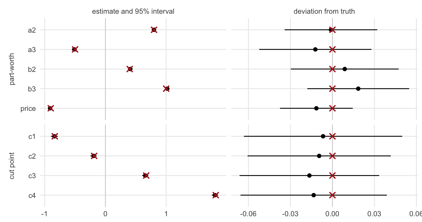
Every \(z\) statistic is small. With nine parameters we would expect roughly one value above two in absolute terms about forty percent of the time.
In [10]:
suppressMessages(library(ggplot2))base <-transform( recovery,parameter =factor(recovery$parameter, levels =rev(recovery$parameter)),kind =factor(rep(c("part-worth", "cut point"), c(length(beta_true), W -1)),levels =c("part-worth", "cut point")))# Two views of the same fit: the natural scale, and the deviation scale where# the intervals are wide enough to read.long <-rbind(transform(base, panel ="estimate and 95% interval",x = estimate,lo = estimate -1.96* std_error,hi = estimate +1.96* std_error,ref = truth),transform(base, panel ="deviation from truth",x = estimate - truth,lo = estimate - truth -1.96* std_error,hi = estimate - truth +1.96* std_error,ref =0))long$panel <-factor(long$panel,levels =c("estimate and 95% interval", "deviation from truth"))ggplot(long, aes(y = parameter)) +geom_vline(xintercept =0, linewidth =0.3, colour ="grey78") +geom_pointrange(aes(x = x, xmin = lo, xmax = hi), size =0.3, linewidth =0.5) +geom_point(aes(x = ref), shape =4, size =2.3, stroke =1.1, colour ="firebrick") +facet_grid(kind ~ panel, scales ="free", space ="free_y", switch ="y") +labs(x =NULL, y =NULL) +theme_minimal(base_size =11) +theme(panel.grid.minor =element_blank(),strip.placement ="outside",strip.text.y.left =element_text(angle =90, colour ="grey30"),strip.text.x =element_text(colour ="grey30"))
Recovery of all nine parameters. Dots and bars are the estimate and its 95% confidence interval; red crosses mark the truth. The right panel repeats the intervals centred on the truth, since at 20,000 tasks they are only two to four percent of the left panel’s range and would otherwise be hidden behind the markers.
Every interval in the right panel covers zero, so no parameter is distinguishable from its true value at conventional levels.
The cut points on the probability scale
Pushing the estimated cut points back through the link turns scale labels into purchase probabilities, with standard errors.
The cut points are fixed across tasks, so a label means the same thing on every screen: a respondent choosing the top box is reporting a purchase probability above 0.848, against a true 0.85.
8. Diagnostics
Is the truth inside the confidence region? Compare twice the log-likelihood gap between the truth and the MLE against a \(\chi^2_9\) critical value.
In [12]:
nll_truth <-negloglik(c(beta_true, cut_to_par(cut_true)), dat)lr <-2* (nll_truth - fit$nll)npar <-length(fit$par)cat(sprintf("LR statistic %.2f vs chi-square(%d) 95%% critical value %.2f -> %s\n", lr, npar, qchisq(0.95, npar),ifelse(lr <qchisq(0.95, npar), "inside the region", "OUTSIDE")))
LR statistic 3.44 vs chi-square(9) 95% critical value 16.92 -> inside the region
Is the information matrix well conditioned? Identification is established analytically in the paper; what this checks is that the implementation inherits it. All eigenvalues positive means the negative-likelihood curves upward in every direction, and the smallest one bounds the precision of the worst-determined parameter combination.