
| configuration | top-2-box, beta | worst cut, beta | omega share, top-2-box | omega share, worst |
|---|---|---|---|---|
| set1_moderate | 1.041 | 1.091 | 0.73 | 0.38 |
| set2_negative | 1.088 | 1.119 | 0.59 | 0.40 |
| set3_stress | 1.152 | 1.327 | 0.59 | 0.19 |
| set4_skewed | 1.080 | 1.125 | 0.48 | 0.20 |
\[ \newcommand{\x}{\mathbf{x}} \newcommand{\bfbeta}{\boldsymbol{\beta}} \newcommand{\betabar}{\bar{\bfbeta}} \newcommand{\bftheta}{\boldsymbol{\theta}} \newcommand{\iid}{\stackrel{iid}{\sim}} \newcommand{\E}{\operatorname{E}} \newcommand{\coloneqq}{\mathrel{:=}} \]
1 Introduction
Consumers are good at indicating which product they like best. They are often less certain about whether they would buy it. Choice-based conjoint analysis, the workhorse of stated-preference measurement in marketing (Allenby et al. 2019), has a device for separating the two: the dual-response format (Brazell et al. 2006). In each task, the consumer first makes a forced choice among the displayed product profiles and then answers a follow-up question about whether she would actually purchase her selection. The format was introduced to fix a practical problem with the traditional no-choice option: tasks in which “none of these” is chosen carry no information about attribute preferences. The dual-response format recovers that lost information because the forced choice always reveals preference among profiles, while still measuring demand for the category through the follow-up question, and it does so without systematically biasing the preference estimates (Brazell et al. 2006; Dhar and Simonson 2003). Following its implementation in Sawtooth Software’s widely used choice-based conjoint (CBC) system (Diener et al. 2006; Sawtooth Software 2017), the dual-response format became common practice in commercial conjoint research. The format was not, however, derived from a behavioral model of the consumer. This paper supplies such a model for an ordinal follow-up. It rationalizes the dual-response format, determines the link function, and extends the purchase question from binary to ordinal.
We start from the behavioral premise that a consumer facing a dual-response conjoint task can indicate her most-preferred product profile in the forced choice, but whether she would purchase her selection concerns a hypothetical future occasion about which she remains uncertain. That second question has traditionally been binary: “would you buy the option you selected above?”, answered yes or no and modeled by pairing a multinomial logit for the forced choice with a binary logit for the purchase question (Diener et al. 2006; Hung, Liu, et al. 2025). But a yes-or-no answer requires the consumer to settle something she has not yet had reason to settle. What she holds is a probability (Manski 1990). A finer scale would ask instead for her degree of conviction, and would carry more information about what she will do. The natural extension is an ordinal dual-response follow-up, “how likely are you to buy the option you selected above?”, answered, e.g., on a five-, seven-, or eleven-point scale from “very unlikely” to “very likely.”
We formalize that uncertainty as a component of utility for the outside good that she has not yet resolved, and, in our primary specification, we let the error components (for both the inside goods and the outside good) be independent Gumbel (McFadden 1981; Train 2009). (Appendix D relaxes independence across goods to any generalized extreme value structure.) Together the behavioral premise and the distributional kernel do two things. First, they deliver a closed-form likelihood: the maximum of Gumbel utilities is itself Gumbel, with location equal to the log-sum inclusive value, and independent of which alternative attains it, so the two responses factor and the model pairs a multinomial logit for the forced choice with a cumulative link for the ordinal report. Second, they make the link complementary log-log. The familiar ordered logit (logistic link) arises instead when the uncertainty is resolved before the follow-up, the assumption underlying the binary dual-response models, which Hung, Liu, et al. (2025) state explicitly. At two scale points the logistic link is the “Unified Model” of Hung, Liu, et al. (2025), equivalently the DR-AnyMax model of Diener et al. (2006) and, once the inclusive value cancels, the single-stage multinomial logit with a no-choice constant (Haaijer et al. 2001). Our model predicts a complementary log-log binary response, so the familiar yes/no follow-up is misspecified (if only mildly) whenever consumers remain uncertain.
We make four contributions. First, we develop the behavioral model: a utility-theoretic account of dual-response conjoint in which outside-good uncertainty is the primitive. That premise rationalizes the design and fixes the link function, and the cumulative-link family it generates contains the existing binary models as the two-point case of the alternative link, so the assumptions underlying those models become explicit and testable. Second, we analyze the information content of the ordinal follow-up: we derive the information a second response of a given length contributes and show that it is always non-negative and never falls when the scale is made finer, extending the binary efficiency results of Brazell et al. (2006) and Hung, Liu, et al. (2025) and providing design guidance on how many scale points to use. Third, we provide estimation routines: maximum likelihood for the aggregate model and a custom Markov chain Monte Carlo sampler for the hierarchical Bayesian model with heterogeneous preferences, including an extension with consumer-specific cut points that accommodates individual differences in scale usage (Greene and Hensher 2010b; Falco et al. 2015). We also express the model in Apollo (Hess and Palma 2019) both as a check on our implementation and as a route for readers already working in that framework. Fourth, we supply evidence: simulation studies that demonstrate parameter recovery and quantify the losses from dichotomization and constant-probability weighting, and an empirical application to a commercial choice-based conjoint study with an ordinal dual response, conducted in partnership with a consumer insights consultancy. Complete replication code accompanies the paper, with each study in the simulation program laid out as an executable notebook.
Several literatures stand behind the model. Marketing work on dual-response and no-choice designs established why asking two questions beats a single question with “none of these” as an option: the preference information in a task survives even when the consumer would not buy. That work set the conventions for estimating such models (Brazell et al. 2006; Diener et al. 2006; Haaijer et al. 2001; Hung, Liu, et al. 2025), and the format itself is still being refined. For example, Schlereth and Skiera (2017) separate the forced and the free questions into blocks and add an adaptive rule for choosing which free questions to ask, which limits context effects and extreme response behavior when willingness to pay is the target. Hung, Kurz, et al. (2025) show that the appeal of the no-buy option shifts as a consumer works through the choice tasks. The opt-out literature in choice modeling documents the consequences of getting the no-buy option wrong: misspecifying it degrades the accuracy of both willingness-to-pay estimates and market-share forecasts (Campbell and Erdem 2019).
The separation of the two decisions is older than the dual-response design. Demand models fit to supermarket scanner data have long estimated whether a household buys in a category separately from which brand it picks, joining the two stages through the inclusive value of the brand-choice stage (Gupta 1988; Bucklin and Gupta 1992). Our second response uses that device on survey data. Our statistical tools come from work on ordered and mixed response formats, from frameworks that handle ratings, rankings, and choices together (Marshall and Bradlow 2002) to ordered-choice models that let different people use the same scale differently (Greene and Hensher 2010b; Falco et al. 2015). Closest to our likelihood is the choice-ordered logit of Webb and Hess (2021), which pairs a multinomial logit with an ordered logit for a rating of the chosen alternative. Their ordinal response grades that alternative’s own utility; ours reports a purchase probability measured against an outside good the consumer has not resolved, which is what puts the no-buy margin into the second response. A parallel literature in transport and environmental valuation asks respondents how certain they are of each choice and models that answer jointly with the choice itself (Hensher et al. 2012; Rose et al. 2015), with Hensher et al. (2012) letting the thresholds vary across respondents as our extension in Section 2.9.1 does. A further literature explains why the follow-up should ask for a probability. A yes/no question forces the consumer to round to zero or one, and Manski (2004) argues that economists should elicit the probability itself. Marketing research made the same case decades earlier: Juster (1966) replaced the yes/no buying-intentions question with an eleven-point probability scale, and Morrison (1979) showed that stated intentions predict purchases only probabilistically, and that the mapping from one to the other depends on context. To our knowledge, no prior work derives the forced choice and the ordinal purchase answer from a single account of the consumer.
Section 2 develops the model and its likelihood, nesting, information, and estimation results; Section 3 reports the simulation study, Section 4 the empirical application, and Section 5 the implications for practice, including scale design; Section 6 concludes. The appendices give the proofs (A), the sampler and marginal-likelihood details (B and C), the extension to correlated alternatives (D), the implementation in Apollo (E), and a worked example of the model at its smallest (F).
2 Model
2.1 Setup
Consumer \(i=1,\ldots,N\) faces choice tasks \(t=1,\ldots,T\). Each task presents a set of “inside” goods \(\mathcal{J}^{+} = \lbrace 1,2,\ldots,J \rbrace\) alongside an “outside” good \(j=0\), so that the full choice set is \(\mathcal{J} = \lbrace 0,1,2,\ldots,J \rbrace\).1 Consumer \(i\) derives utility \(u_{itj}\) from good \(j\) in task \(t\): \[ u_{itj} = h(\x_{tj}, \bfbeta_i) + \eta_{itj}, \tag{1}\] where \(\x_{tj}\) is a length-\(P\) column vector of good characteristics, \(\bfbeta_i\) is a length-\(P\) column vector of consumer-specific taste parameters, and \(\eta_{itj}\) encapsulates factors known to the consumer but unobserved by the researcher. We take \(h(\x_{tj}, \bfbeta_i) = \x_{tj}'\bfbeta_i\) and write \(V_{itj} \coloneqq \x_{tj}'\bfbeta_i\) for this deterministic component, but the linear specification is not required.
The outside good is special in two respects. First, it is associated with a zero vector of characteristics (\(\x_{t0} = \mathbf{0}\)), so that \(V_{it0}=0\); this is the standard normalization that anchors the location of utility (Haaijer et al. 2001). Second, and this is the paper’s central behavioral assumption, the consumer observes \(\eta_{itj}\) for all inside goods but does not observe \(\eta_{it0}\). The outside good stands in for a purchase occasion that has not yet arrived, and her evaluation of it is uncertain.2 3
In each task the consumer provides two responses:
First response (choice). She reports her preferred inside good, \[ j^*_{it} = \underset{j \in \mathcal{J}^+}{\operatorname{arg max}} \ u_{itj}. \tag{2}\] This is a forced choice: the outside good is not among the options.
Second response (the ordinal report). She reports a value \(y_{it}\) on a discrete ordinal scale \(w \in \mathcal{W} = \lbrace 1, \ldots, W \rbrace\) (e.g., “very unlikely” to “very likely” on a five-point scale) that characterizes her evaluation of purchasing \(j^*_{it}\), that is, of choosing it over the outside good. The binary dual-response format of Brazell et al. (2006) and Diener et al. (2006) is the special case \(W=2\) of this design.
We model \(\eta_{itj} \iid \text{Gumbel} \left( 0,1 \right)\), independent of \(\x_{tj}\) and independent across goods, tasks, and consumers. This is the logit kernel standard in discrete choice (McFadden 1981; Train 2009), inherited by choice-based conjoint. The independence across goods is stronger than our derivation needs. Appendix D shows that Lemma 1 holds for any generalized extreme value error structure once \(S_{it}\) is replaced by the GEV generator, so the following results carry over to correlated alternatives, but for exposition we proceed with the independent errors assumption.
Two classical properties of the Gumbel family are used throughout (McFadden 1981).
Lemma 1 Let \(u_{itj} = V_{itj} + \eta_{itj}\) with \(\eta_{itj} \iid \text{Gumbel}(0,1)\) for \(j \in \mathcal{J}^+\), and define \(u^*_{it} = \max_{j \in \mathcal{J}^+} u_{itj}\). Then
\(u^*_{it} \sim \text{Gumbel}\left(\overline{\mu}_{it}, 1\right)\) with location \[ \overline{\mu}_{it} = \ln S_{it}, \qquad S_{it} \coloneqq \sum_{j\in\mathcal{J}^{+}} \exp \left( V_{itj} \right); \tag{3}\]
the identity of the maximizer \(j^*_{it}\) and the value of the maximum \(u^*_{it}\) are statistically independent.
Property (ii) makes the dual-response likelihood tractable: whatever the consumer tells us about the level of her best utility (the second response) is independent of which good delivered it (the first response), conditional on the deterministic utilities. Both properties are standard; Appendix A reproduces the short derivation.
2.2 First Response: Multinomial Logit
The first response is a standard forced choice among the inside goods. Under the Gumbel assumption, \[ \Pr \left( j^*_{it} = j \right) = \frac{\exp \left( V_{itj} \right)}{\sum_{k\in\mathcal{J}^{+}} \exp \left( V_{itk} \right)} = \frac{\exp \left( V_{itj} \right)}{S_{it}}, \tag{4}\] the multinomial logit over inside goods only. The outside good does not appear: the forced choice does not depend on the consumer’s uncertain evaluation of the outside good, which is the design’s appeal (Brazell et al. 2006).
2.3 Second Response: An Ordinal Model of the Purchase Report
Our premise determines what the consumer consults when answering “how likely are you to purchase the option you selected?”: she has not resolved \(\eta_{it0}\), so what she has to report is a probability. That premise delivers a likelihood of cumulative-link form, depending on the choice set only through the inclusive value \(\overline{\mu}_{it}\), and it determines the link.
She knows \(u^*_{it}\) (she just identified \(j^*_{it}\)) but does not know \(\eta_{it0}\), so from her perspective the probability that she would follow through and purchase \(j^*_{it}\) is \[ p_{it} = \Pr \left( \eta_{it0} < u^*_{it} \mid u^*_{it} \right) = F\left( u^*_{it} \right), \tag{5}\] where \(F(z) = \exp(-e^{-z})\) is the standard Gumbel CDF. The ordinal scale discretizes the unit interval: fix cut points \(0 = \alpha_0 < \alpha_1 < \cdots < \alpha_{W-1} < \alpha_W = 1\) and suppose the consumer reports \[ y_{it} = w \quad \Longleftrightarrow \quad p_{it} \in \left[ \alpha_{w-1}, \alpha_w \right). \tag{6}\] We assume consumers share the definitions of the qualitative scale labels, so the \(\alpha_w\) are common across consumers (we relax this in Section 2.9.1); the interior cut points are unobserved by the researcher and are estimated.
Reporting \(y_{it}=w\) is equivalent to reporting that \(u^*_{it} \in \left[ F^{-1}(\alpha_{w-1}), \, F^{-1}(\alpha_w) \right)\), an interval statement about the consumer’s best utility. From the researcher’s perspective, \(u^*_{it} \sim \text{Gumbel}(\overline{\mu}_{it},1)\) by Lemma 1(i), so \[ \begin{aligned} \Pr \left( y_{it} = w \right) &= F_{\text{Gumbel}(\overline{\mu}_{it},1)} \left( F^{-1}(\alpha_w) \right) - F_{\text{Gumbel}(\overline{\mu}_{it},1)} \left( F^{-1}(\alpha_{w-1}) \right) \\ &= \alpha_w^{\,S_{it}} - \alpha_{w-1}^{\,S_{it}}, \end{aligned} \tag{7}\] To see this, drop subscripts and note \(F_{\text{Gumbel}(\overline{\mu},1)}(z) = \exp\left( -e^{-(z - \overline{\mu})} \right) = \exp\left( -e^{-z}S \right) = \left[ \exp\left( -e^{-z} \right) \right]^{S} = F(z)^{S}\) with \(S = e^{\overline{\mu}}\). Evaluate that at \(z = F^{-1}(\alpha)\), where \(F(z) = \alpha\) by definition, and what is left is \(\alpha^{S}\). The second-response probabilities are differences of powers of the cut points, with the exponent \(S_{it} = e^{\overline{\mu}_{it}}\) summarizing the attractiveness of the task’s inside goods: the more attractive the set, the more probability mass shifts toward high scale points.4
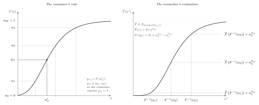
The second-response probabilities are differences of powers of the cut points, with the exponent \(S_{it} = e^{\overline{\mu}_{it}}\) summarizing the attractiveness of the task’s inside goods: the more attractive the set, the more probability mass shifts toward high scale points.5
The distribution’s mean is \(\E \left[ p_{it} \right] = S_{it} \big/ \left( S_{it} + 1 \right) = \Lambda \left( \overline{\mu}_{it} \right)\): averaged over everything the researcher cannot see, the probability of purchase is the logistic of the inclusive value, \(\Lambda(z) = 1 \big/ \left( 1 + e^{-z} \right)\). Conditioning on what she reported rescales it. A consumer who answers \(w\) has \[ \E \left[ p_{it} \mid y_{it} = w \right] = \frac{S_{it}}{S_{it}+1} \cdot \frac{\alpha_w^{\,S_{it}+1} - \alpha_{w-1}^{\,S_{it}+1}}{\alpha_w^{\,S_{it}} - \alpha_{w-1}^{\,S_{it}}}, \tag{8}\] the unconditional mean times a correction for the bin. Because \(S_{it}\) appears here as well as in the bin boundaries, the same scale point implies different purchase probabilities in different tasks: what a label is worth depends on what was on the screen.
It will be convenient to carry these thresholds on two scales. On the probability scale they are directly interpretable: \(\alpha_w\) is the purchase probability at which the consumer moves from label \(w\) to label \(w+1\). On the utility scale, written \(c_w = F^{-1}(\alpha_w)\), they sit alongside \(\overline{\mu}_{it}\) and cast Equation 7 as a cumulative link in the inclusive value, \[ \Pr \left( y_{it} \le w \right) = F \left( c_w - \overline{\mu}_{it} \right). \tag{9}\] Ours is the complementary log-log link, inherited from the Gumbel kernel. We state the model in \(\boldsymbol{\alpha}\), which is what an application reports, and work in \(\mathbf{c}\) wherever the argument concerns the location of \(\overline{\mu}_{it}\), because a common shift in utilities is additive in \(\mathbf{c}\) and a power in \(\boldsymbol{\alpha}\).
2.4 Joint Likelihood
By Lemma 1(ii), the value of \(u^*_{it}\) is independent of the identity of \(j^*_{it}\); and \(\eta_{it0}\) is independent of the inside-good components. The two responses in a task are therefore independent conditional on \((\x_t, \bfbeta_i)\), and the per-task likelihood contribution is the product of Equation 4 and Equation 7: \[ L_{it} \left( \bfbeta_i, \boldsymbol{\alpha} \right) = \underbrace{\frac{\exp \left( V_{itj^*} \right)}{S_{it}}}_{\text{choice}} \; \times \; \underbrace{\left( \alpha_{y_{it}}^{\,S_{it}} - \alpha_{y_{it}-1}^{\,S_{it}} \right)}_{\text{ordinal report}}, \tag{10}\] with \(\boldsymbol{\alpha} = (\alpha_1, \ldots, \alpha_{W-1})\), and the consumer’s likelihood \(L_i = \prod_{t} L_{it}\). The same product form appears in the choice-ordered logit of Webb and Hess (2021), where it follows from treating choice and rating as separate steps. Here it is not an assumption: the two responses are generated by the same utility draw, and Lemma 1(ii) makes them independent anyway.
The per-task log-likelihood is \[ \ell_{it} = \underbrace{V_{itj^*} - \overline{\mu}_{it}}_{\text{choice}} \; + \; \underbrace{\ln \left( \alpha_{y_{it}}^{\,S_{it}} - \alpha_{y_{it}-1}^{\,S_{it}} \right)}_{\text{ordinal report}}, \tag{11}\] with the sample log-likelihood \(\ell = \sum_i \sum_t \ell_{it}\). The forced choice contributes the chosen good’s utility measured against the inclusive value, so a task adds more to the log-likelihood the more the chosen good stands out from the set. The ordinal report contributes the log of the mass Equation 7 puts in the reported bin, so it adds most when the attractiveness of the set sits in that bin: a report near the top of the scale pulls \(\overline{\mu}_{it}\) up, and a report near the bottom pulls it down.6 The first term captures only how the goods compare with one another; the second depends only on where they sit as a group.
2.5 Special Cases and Relation to Existing Models
The resolved comparison. The existing binary dual-response models rest on a different premise: that the consumer resolves the outside-good shock before answering, and so evaluates the realized difference \(d_{it} = u^*_{it} - \eta_{it0}\). Hung, Liu, et al. (2025) state the premise explicitly, specifying that consumers bring the same private information to both responses, and derive the binary case from it; Diener et al. (2006) reach the same functional form by a different route. A consumer in this position can supply the sign of \(d_{it}\), which is all a binary follow-up asks of her. Carried to a \(W\)-point scale the construction is harder to read, since having resolved the comparison she has no likelihood left to report and a graded answer would be something like an intensity rather than a probability; but it remains mathematically well defined, and we use it both for the \(W=2\) result below and as the misspecified link in Section 3.5. Fix utility-scale cut points \(-\infty = c_0 < c_1 < \cdots < c_{W-1} < c_W = \infty\) and suppose \(y_{it} = w\) exactly when \(d_{it} \in \left[ c_{w-1}, c_w \right)\). From the researcher’s perspective \(u^*_{it} \sim \text{Gumbel}(\overline{\mu}_{it},1)\) and \(\eta_{it0} \sim \text{Gumbel}(0,1)\) are independent, so their difference is logistic, \(d_{it} \sim \text{Logistic}\left( \overline{\mu}_{it}, 1 \right)\), and \[ \Pr \left( y_{it} = w \right) = \Lambda \left( c_w - \overline{\mu}_{it} \right) - \Lambda \left( c_{w-1} - \overline{\mu}_{it} \right). \tag{12}\] This is an ordered logit (Greene and Hensher 2010a) in the inclusive value: Equation 9 with the logistic CDF \(\Lambda\) in place of our \(F\). Figure 2 sets the two rules side by side; they share the forced choice and differ only in whether \(\eta_{it0}\) is resolved before or after the report.
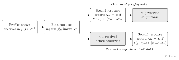
Binary dual response, logistic link. Set \(W=2\), writing the single cut point as \(c_1 = \gamma\). Then \(\Pr(\text{would buy}) = \Lambda\left( \overline{\mu}_{it} - \gamma \right) = S_{it} \big/ \left( e^{\gamma} + S_{it} \right)\), and the joint probabilities from Equation 10 reduce to: \[ \Pr \left( j, \text{buy} \right) = \frac{\exp \left( V_{itj} \right)}{e^{\gamma} + S_{it}}, \qquad \Pr \left( j, \text{not buy} \right) = \frac{\exp \left( V_{itj} \right)}{S_{it}} \cdot \frac{e^{\gamma}}{e^{\gamma} + S_{it}}. \tag{13}\] With \(\gamma = 0\) these are exactly the joint probabilities of the “Unified Model” of Hung, Liu, et al. (2025) (their Eq. 4), which is in turn algebraically identical to the “DR-AnyMax” model of Diener et al. (2006); and Equation 13 with free \(\gamma\) is the standard single-stage MNL with a no-choice alternative-specific constant (Haaijer et al. 2001). The incumbent binary model is therefore the two-point, logistic case of Equation 9; for \(W>2\) the additional cut points are the only new parameters.
Binary dual response, our model. Set \(W=2\) in Equation 7: \(\Pr(\text{not buy}) = \alpha_1^{S_{it}} = F\left( c_1 - \overline{\mu}_{it}\right)\), a complementary log-log rather than logistic binary response. Our model therefore implies that when consumers face outside-good uncertainty at the moment they answer, the familiar (logistic) binary dual response model is misspecified, if only mildly, since the two links are close.
DR-2Max. The other binary model in the literature, “DR-2Max” (Diener et al. 2006), as implemented in Sawtooth Software’s CBC/HB (Sawtooth Software 2017), models the second response as a binary logit on the chosen good’s deterministic utility: \(\Pr(\text{buy} \mid j^*) = e^{V_{itj^*}} \big/ \left( e^{V_{itj^*}} + e^{\gamma} \right)\). This implies drawing a fresh error for the chosen good in the second stage, so that the consumer who just declared \(j^*\) best re-evaluates it from scratch. Under our framework such conditioning is unnecessary: by Lemma 1(ii) the distribution of the best utility does not depend on which good attained it, so the second response should depend on the set only through \(\overline{\mu}_{it}\). The same conditioning, generalized from a binary follow-up to an ordinal rating, is the two-step choice-ordered logit of Webb and Hess (2021), whose second stage is an ordered logit in \(\zeta V_{itj^*}\) with a free scale \(\zeta\). That specification is therefore the \(\delta = 1\) end of the conditioning test of Section 2.7, and our \(\lambda\) plays the role of their \(\zeta\) on the inclusive value rather than on the chosen good.
Reductions to the binary model. An ordinal response can be reduced to a form the binary model accepts in two ways: (i) dichotomization, collapsing the scale at some point (e.g., top box or top two boxes) and estimating the binary model, which discards the ordinal information and hard-codes an arbitrary cut; or (ii) constant-probability weighting, mapping each scale point to a fixed purchase probability (e.g., “definitely would buy” \(= 0.9\)) independent of the choice set. These two reductions are the benchmarks in our simulation study (Section 3). Both are nested within, or dominated by, Equation 10: dichotomization is Equation 13 applied to a coarsened \(y_{it}\), and constant-probability weighting fixes the value of a scale point, which by Equation 8 varies with the task through \(S_{it}\) (i.e., constant-probability weighting is inappropriate since no single value assigned to a scale point is right for every task).
2.6 Identification
Because the second response depends on the choice set only through the log-sum \(\overline{\mu}_{it}\), and because the cut points sit on the same utility scale as \(\overline{\mu}_{it}\), the model requires a location normalization. Fix the aggregate model (\(\bfbeta_i = \bfbeta\)) and let a task \(t\) have inside-good attribute vectors \(\lbrace \x_{tj} \rbrace_{j \in \mathcal{J}^+}\) and responses \(\left( j^*_t, y_t \right)\) generated by Equation 10 with parameter \(\theta = \left( \bfbeta, \mathbf{c} \right) \in \mathbb{R}^P \times \mathcal{C}\), where \(\mathcal{C} = \lbrace \mathbf{c} : c_1 < \cdots < c_{W-1} \rbrace\). Call \(\theta\) and \(\theta'\) observationally equivalent if they imply the same joint probabilities \(\Pr_\theta \left( j^*_t = j, y_t = w \right)\) for every task design in the support of the design distribution, and let \(X\) denote the design matrix that stacks the rows \(\x_{tj}'\) over all inside goods and tasks in that support.
Proposition 1 \(\theta = \left( \bfbeta, \mathbf{c} \right)\) is identified if and only if the augmented matrix \(\left[ X \;\; \iota \right]\) has full column rank \(P+1\), where \(\iota\) is a conformable vector of ones. Equivalently: the only \(\left( v, \delta \right) \in \mathbb{R}^P \times \mathbb{R}\) satisfying \(\x_{tj}'v = \delta\) for every inside good \(j\) and task \(t\) is \(\left( v, \delta \right) = \left( \mathbf{0}, 0 \right)\).
Proof. (Sufficiency.) Suppose \(\theta\) and \(\theta' = \left( \bfbeta', \mathbf{c}' \right)\) are observationally equivalent. Marginalizing the joint probabilities over \(y\) equates the MNL choice probabilities task by task, which implies \(\left( \x_{tj} - \x_{tk} \right)' \left( \bfbeta - \bfbeta' \right) = 0\) for all \(j,k,t\); hence \(\x_{tj}' \left( \bfbeta - \bfbeta' \right) = a_t\), a constant within each task. Marginalizing over \(j\) equates the cumulative ordinal probabilities: \(F \left( c_w - \overline{\mu}_t(\bfbeta) \right) = F \left( c'_w - \overline{\mu}_t(\bfbeta') \right)\) for all \(w,t\). Since \(F\) is strictly increasing, \(c_w - c'_w = \overline{\mu}_t(\bfbeta) - \overline{\mu}_t(\bfbeta')\) for all \(w,t\); the left side is free of \(t\) and the right side free of \(w\), so both equal a constant \(\delta\). Direct computation gives \(\overline{\mu}_t(\bfbeta') = \ln \sum_j \exp \left( V_{tj} - a_t \right) = \overline{\mu}_t(\bfbeta) - a_t\), so \(a_t = \delta\) for every \(t\); that is, \(\x_{tj}' \left( \bfbeta - \bfbeta' \right) = \delta\) for all \(j,t\). The rank condition then forces \(\bfbeta = \bfbeta'\) and \(\delta = 0\), hence \(\mathbf{c} = \mathbf{c}'\). (Necessity.) If some \(\left( v, \delta \right) \ne \left( \mathbf{0}, 0 \right)\) satisfies \(\x_{tj}'v = \delta\) everywhere, then \(\theta' = \left( \bfbeta + v, \mathbf{c} + \delta \iota \right)\) shifts every \(V_{tj}\) and every cut point by \(\delta\), leaving the MNL probabilities (a within-task constant drops out) and the ordinal probabilities (\(F(c_w + \delta - (\overline{\mu}_t + \delta))\)) unchanged, so \(\theta' \ne \theta\) is observationally equivalent to \(\theta\). \(\square\)
The condition in miniature. Return to the two consumers of Appendix F, with \(\beta = 1\) and \(\mathbf{c} = (0,2)\), so that \(\overline{\mu}_1 = 2.31\) and \(\overline{\mu}_2 = -0.69\). Suppose the design had carried a constant: one extra attribute, equal to one for every good, with part-worth \(\beta_{\text{const}}\). Setting \(\beta_{\text{const}} = 1\) raises every \(V_{tj}\) by one and therefore raises both inclusive values by exactly one, to \(3.31\) and \(0.31\). Raise both cut points by one as well, to \(\mathbf{c} = (1,3)\), and every difference \(c_w - \overline{\mu}_t\) returns to the value it had: \((-2.31, -0.31)\) for the first consumer and \((0.69, 2.69)\) for the second. The two ordinal distributions are therefore unchanged. The forced choice never saw the constant at all, since it turns on \(\x_{t1} - \x_{t2}\). No quantity of data separates \(\left( \beta_{\text{const}}, \mathbf{c} \right) = \left( 0, (0,2) \right)\) from \(\left( 1, (1,3) \right)\), or from any other point along that ridge, on which the cut points move one for one with the constant.
Several remarks unpack Proposition 1.
What the condition rules out. A violating direction \(\left( v, \delta \right)\) is an attribute combination whose value is the same for every inside good ever shown. The leading case is an intercept: a column of ones in \(X\) makes \(\left[ X \;\; \iota \right]\) rank deficient by construction. The subtler case is a hidden intercept: if an attribute is dummy-coded with all \(L\) of its levels included, every alternative carries exactly one of them, so the dummies sum to \(\iota\) and the same invariance appears (shift all \(L\) part-worths and all cut points equally). Attributes must therefore be coded against omitted reference levels (or effects-coded), and the design must contain no global constant. This requirement is stricter than in the single-stage MNL with a no-choice alternative, where a full set of brand dummies is identified because the no-choice row of zeros breaks the constancy (Haaijer et al. 2001). In the dual-response model the outside good never appears as a design row, since its role is absorbed by the cut points, so anything the design holds constant across inside goods is absorbed along with it.
What the normalizations do. The convention \(\x_{t0} = \mathbf{0}\) with a \(\text{Gumbel}(0,1)\) shock fixes the origin against which the cut points are measured: an outside-good alternative-specific constant would shift all cut points equally, which is the invariance in the proof, so the cut points subsume it. (Its visible trace is the binary case: at \(W=2\), the logistic link’s single cut point \(c_1\) is the no-choice constant of Equation 13.) The unit Gumbel scale fixes the scale of \(\bfbeta\), as in any logit. Beyond these normalizations, the model imposes one restriction: the coefficient on \(\overline{\mu}_{it}\) in Equation 9 is fixed at \(1\) by the theory, because both responses are driven by the same utility draw. Estimating a free slope \(\lambda\) on \(\overline{\mu}_{it}\) and testing \(\lambda = 1\) is therefore an overidentification test of the behavioral model (Section 2.7).
Cut points versus the link. Given \(\bfbeta\) (identified from the forced choice alone whenever \(X\)’s within-task differences have full rank), the cut points are exactly identified even without variation in task attractiveness: \(c_w = \overline{\mu} + F^{-1} \left( \Pr(y \le w) \right)\) pointwise. Because \(\bfbeta\) fixes each task’s inclusive value, we can read a cut point straight off the frequency of the categories it bounds: if 30% of reports in a task fall at or below \(w\), then \(c_w\) is the threshold satisfying \(F \left( c_w - \overline{\mu} \right) = 0.30\). One task supplies \(W-1\) independent cumulative frequencies for the \(W-1\) free cut points, so the count is exact. Variation in \(\overline{\mu}_{it}\) across tasks therefore overidentifies \(\mathbf{c}\), and it is what identifies the link: at a single value of \(\overline{\mu}\), any two strictly increasing links fit the \(W\) category frequencies perfectly by relabeling cut points, so the shape of the link is identified only through how the ordinal distribution shifts as \(S_{it}\) varies. Designs that hold task attractiveness fixed cannot speak to it at all.
Population versus sample. Under Proposition 1 every scale category has strictly positive probability in every task (\(F\) is strictly increasing on \(\mathbb{R}\) and the cut points are finite), so no support condition is needed for point identification. In finite samples, however, rarely used categories leave their adjacent cut points weakly identified, and near-violations of the rank condition (attribute combinations nearly constant across inside goods) manifest as an ill-conditioned information matrix. Both pathologies are visible in the smallest eigenvalues of the observed information, a diagnostic we report alongside the simulation results in Section 3.
Numerical demonstration. The proof settles Proposition 1; simulation instead checks that our likelihood and estimation code behave as it describes, and makes the predicted failure concrete (replication code accompanies the paper). Data simulated from the raw behavioral process (Gumbel utility draws, argmax, and the two reporting rules, not the derived likelihood) at three distinct parameter configurations for each model, on designs satisfying the rank condition, are recovered by maximum likelihood: across all configurations the true parameter vector lies inside the 95% likelihood-ratio confidence region, the observed information is well-conditioned, repeated-sampling bias is statistically indistinguishable from zero, and model-based standard errors match the empirical sampling variation. Appending an intercept column, the canonical violation, produces the predicted failure: \(\left[ X \;\; \iota \right]\) loses rank, the smallest eigenvalue of the observed information collapses to zero, and different starting values converge to different raw \(\left( \beta_{\text{const}}, \mathbf{c} \right)\) on the flat ridge while agreeing, to numerical precision, on the identified combinations \(c_w - \beta_{\text{const}}\) and the non-constant coordinates of \(\bfbeta\). The same exercise confirms the factorization in Equation 10: the empirical joint distribution of \(\left( j^*, y \right)\) from one million behavioral draws is statistically indistinguishable from the product form.
2.7 Specification Tests
Because the theory restricts more than it parameterizes, the model is overidentified in two directions that convert directly into one-degree-of-freedom specification tests. Both are computed from the aggregate likelihood at trivial cost, and both have well-behaved operating characteristics (Section 3).
The unit-slope test. The behavioral model fixes the coefficient on the inclusive value in the second stage at exactly one, because the same utility draw generates both responses, so the natural one-parameter enlargement \[ \Pr \left( y_{it} \le w \right) = F \left( c_w - \lambda \, \overline{\mu}_{it} \right) \tag{14}\] nests the model at \(\lambda = 1\). A free \(\lambda\) is identified by how the ordinal response distribution shifts as task attractiveness varies (Section 2.6), and departures are interpretable: \(\lambda < 1\) indicates the second response under-reacts to the quality of the displayed set (consistent with inattention to the set or with scale-use compression), while \(\lambda > 1\) indicates over-reaction. Testing \(H_0\!: \lambda = 1\) by likelihood ratio or Wald therefore tests the joint utility account.
The conditioning test. The framework implies the second response depends on the choice set only through \(\overline{\mu}_{it}\) (Lemma 1), whereas the DR-2Max tradition conditions on the chosen alternative’s utility. The enlargement \[ \Pr \left( y_{it} \le w \right) = F \left( c_w - \left[ \overline{\mu}_{it} + \delta \left( V_{itj^*} - \overline{\mu}_{it} \right) \right] \right) \tag{15}\] spans the two: \(\delta = 0\) is our model and \(\delta = 1\) puts the full weight on the chosen option’s deterministic utility, the DR-2Max predictor. The bracket is \((1-\delta) \overline{\mu}_{it} + \delta V_{itj^*}\), so \(\delta\) is that weight. Both points are testable against the estimated \(\delta\), so the long-standing 2Max-versus-AnyMax question (Diener et al. 2006; Hung, Liu, et al. 2025) becomes a parameter estimate rather than a model-selection exercise.
We apply both tests to the empirical data in Section 4. The simulation study documents their finite-sample size and power, including full power of the \(\delta\) test against DR-2Max data at modest sample sizes.
2.8 The Information Content of the Ordinal Response
We measure what a \(W\)-point second response adds over a binary one by its Fisher information, which extends the efficiency analysis of Hung, Liu, et al. (2025) from binary to ordinal second responses.
The per-task Fisher information about \(\bfbeta\) decomposes into the familiar MNL term (Huber and Zwerina 1996) plus a second-response increment. Writing \(\pi_w = F(c_w - \overline{\mu}) - F(c_{w-1} - \overline{\mu})\) and \(f = F'\), the second response contributes \[ \mathcal{I}^{(2)}_{it} = \omega \left( \overline{\mu}_{it}; \mathbf{c} \right) \, \overline{\x}_{it} \, \overline{\x}_{it}', \qquad \omega = \sum_{w=1}^{W} \frac{ \left[ f \left( c_w - \overline{\mu} \right) - f \left( c_{w-1} - \overline{\mu} \right) \right]^2 }{ \pi_w }, \tag{16}\] where \(\overline{\x}_{it} = \sum_{j \in \mathcal{J}^+} \Pr\left(j^*_{it}=j\right) \x_{tj}\) is the choice-probability-weighted average attribute vector (the gradient of \(\overline{\mu}_{it}\) with respect to \(\bfbeta\)). Two properties follow. First, the increment is positive semi-definite: the second response never destroys information, as in the binary result of Hung, Liu, et al. (2025). Second, \(\omega\) is non-decreasing under refinement of the scale partition: merging two adjacent categories pools their scores, and by Cauchy–Schwarz the pooled cell contributes no more than the two it replaces (Appendix A). The binary response (\(W=2\)) is therefore the least informative member of the family, and information rises toward the continuous-report limit as \(W \to \infty\). Section 3 quantifies the practical magnitudes: how much of the binary-to-continuous gap a five- or seven-point scale captures, and how the gains vary with task attractiveness.
2.9 Heterogeneity
We accommodate preference heterogeneity with a standard hierarchical Bayesian specification (Rossi et al. 2005; Train 2001): \[ \bfbeta_i \iid \mathcal{N} \left( \betabar, \Sigma_{\beta} \right), \tag{17}\] with conjugate priors on \(\left( \betabar, \Sigma_{\beta} \right)\). In the main model the cut points \(\mathbf{c}\) are common across consumers: the scale labels (“very likely,” “somewhat likely,” …) are assumed to mean the same thing to everyone, while preferences vary.
2.9.1 Heterogeneous Cut Points
The assumption of a shared reporting scale is convenient but contestable: Greene and Hensher (2010a) and Falco et al. (2015) document individual differences in the use of ordinal response scales. We therefore develop an extension with consumer-specific cut points. Parameterize \[ c_{i1} \in \mathbb{R}, \qquad c_{iw} = c_{i,w-1} + \exp \left( \delta_{iw} \right) \ \text{for} \ w = 2, \ldots, W-1, \tag{18}\] and let \(\bftheta_i = \left( c_{i1}, \delta_{i2}, \ldots, \delta_{i,W-1} \right)'\) follow a multivariate normal population distribution, estimated jointly with (and, if desired, correlated with) \(\bfbeta_i\). The exponentiated increments enforce monotonicity without constrained sampling. Identification at the individual level is necessarily partial, because with \(T\) tasks per consumer the \(W-1\) individual cut points and \(P\) individual preference parameters are jointly informed by only \(T\) ordinal reports. The hierarchy matters here because it shrinks each consumer’s scale usage toward a population distribution that is estimated from the whole sample. Section 3 examines both the payoff to permitting cut-point heterogeneity when it is present in the data-generating process and the robustness of the common-cut-point model when it is not.
Identification with heterogeneity. Proposition 1 applies consumer by consumer once \(\bfbeta_i\) varies: individual-level identification requires the rank condition on each consumer’s own stacked design (her \(T \times J\) rows), which rotating commercial designs typically satisfy. The hierarchy then supplies shrinkage, not identification of the model’s fixed features. In the heterogeneous-cut-point extension, the same location tension reappears at the individual level, where a consumer-specific utility shift trades off against \(c_{i1}\) within that consumer’s likelihood, and is resolved by the same condition applied to the individual design, and the hierarchical prior matters most when \(T\) is small.
2.10 Estimation
The aggregate (homogeneous-\(\bfbeta\)) model is estimated by maximum likelihood: the log of Equation 10 summed over consumers and tasks is smooth in \(\left( \bfbeta, \mathbf{c} \right)\) after the monotonicity-preserving reparameterization of the cut points, and standard quasi-Newton methods converge quickly. One term needs care. When a scale point is rarely used, the two powers in Equation 11 differ only in a late decimal place, and subtracting them as written would discard most of the precision the computer has; the code evaluates an algebraically identical rearrangement that never forms that difference (Appendix B). Because the likelihood is a product of a choice component and an ordinal component, it can also be assembled in Apollo (Hess and Palma 2019) from that package’s standard building blocks, which we do as an independent check on our own code. Appendix E gives the details.
The hierarchical model is estimated with a custom Markov chain Monte Carlo sampler, implemented in R and following the hybrid Gibbs architecture of Rossi et al. (2005): (1) a random-walk Metropolis step for each \(\bfbeta_i\) (and \(\bftheta_i\) in the heterogeneous-cut-point extension) using the individual likelihood \(\prod_t L_{it}\); (2) a random-walk Metropolis step for the common cut-point block on the unconstrained scale; and (3) conjugate draws for the population moments \(\left( \betabar, \Sigma_{\beta} \right)\). Model comparison uses the log marginal density approximated by the method of Newton and Raftery (1994), matching the practice in Hung, Liu, et al. (2025) and permitting direct comparisons among our model, the binary dual-response models, and the practitioner heuristics. Complete replication code accompanies the paper.
3 Simulation Study
The simulation program serves six purposes: verify that the estimators recover the model’s parameters and check the identification theory of Section 2.6, including the failure it predicts; quantify what dichotomization costs, in the aggregate and, where it matters more, at the individual level; establish the operating characteristics of the specification tests of Section 2.7; probe robustness to plausible misspecifications; turn the information results of Section 2.8 into design guidance; and attach economic stakes to the choice of estimator through a pricing counterfactual.
Two conventions apply throughout. We simulate all data from the behavioral process (raw Gumbel utility draws, the argmax, and the reporting rules), never from the derived likelihood, so parameter recovery checks the derivation and the code at once. Every experiment is seeded and reproducible.
Each subsection below summarizes one study and points to its notebook. The notebooks run the experiments end to end and produce every number reported here; they also carry the diagnostics, intermediate tables, and negative controls not worth article space. Readers who want to see a result rather than take it on trust should start there.
3.1 Design
The aggregate experiments pool tasks with \(J = 4\) alternatives described by two 3-level attributes (dummy-coded against reference levels) and a continuous price-like attribute (\(P = 5\)). The second response uses a \(W = 5\) scale, and four parameter configurations vary the location and spread of the response distribution. One is a skewed configuration with realistic bottom-heavy purchase intent (top-2-box share 18.4%), where the top-2-box convention is worst placed. The hierarchical experiments use \(N = 300\) consumers, \(T = 12\) estimation tasks plus 2 holdouts, \(\bfbeta_i \sim \mathcal{N}(\betabar, \Sigma)\) with substantial heterogeneity, and the same attribute scheme. Attribute levels are drawn at random rather than from an efficiency-optimized catalogue. The comparisons that carry the results are paired, with competing specifications fit to the same simulated data, so design efficiency cancels from them, and the rank condition of Proposition 1 is checked before every fit. Optimizing for the forced choice alone would not in any case serve the second response, which is identified by variation in task attractiveness across tasks rather than by the within-task contrasts that utility balance equalizes (Huber and Zwerina 1996); what an efficient design for a dual-response instrument looks like is an open question.
3.2 Parameter Recovery and Identification
Aggregate. Notebook 2 runs three parameter configurations per link at 20,000 tasks each. In every case the true parameter vector lies inside the 95% likelihood-ratio confidence region, the observed information is strongly positive definite, and the probability-scale cut points of our model recover to within a percentage point: a true \(\alpha_1 = 0.02\) in the stress configuration is estimated at 0.0196. Repeated-sampling behavior matches the asymptotics. Across 40 independent datasets per link at \(n = 5{,}000\), no parameter shows significant bias (max \(|t| = 2.05\) over 18 tests) and model-based standard errors match the empirical sampling variation (mean calibration ratio 1.008). Quadrupling \(n\) shrinks the largest observed bias in proportion, as ordinary \(O(1/n)\) finite-sample bias would.
The same notebook runs the two numerical checks summarized in Section 2.6. Appending an intercept, the canonical violation of Proposition 1, collapses the smallest eigenvalue of the observed information and produces the predicted flat ridge: different starting values reach identical likelihoods at different raw \((\beta_{\text{const}}, \mathbf{c})\) — spread 1.00 across starts — while agreeing on the identified combinations to within 1e-07. And the empirical joint distribution of the two responses over one million behavioral draws is statistically indistinguishable from the product form of Equation 10, confirming the factorization that makes the likelihood tractable.
Hierarchical. Notebook 3 establishes that the sampler of Section 2.10 recovers population means, covariances, and cut points on synthetic panels, and that its posterior uncertainty is calibrated: across 8 replications, 90% central posterior intervals cover the truth at 89% (resolved comparison) and 83% (our model), with 50% intervals at 51% and 43%. Calibration matters independently of recovery, since a sampler can find the right answer and still misstate its own uncertainty. As a check on the hierarchical code, the forced-choice-only special case of our sampler agrees with an established hierarchical-MNL implementation on identical data to within 0.007 on every population parameter.
3.3 The Cost of Dichotomization
Collapsing the \(W\)-point response at a cut point yields a correctly specified binary dual-response model, so dichotomization costs efficiency and never consistency; notebook 4 confirms this with bias tests in every cell. The comparison is therefore about precision, and we compute it two ways: exactly, from the Fisher information, and by paired Monte Carlo, fitting the ordinal model and the binary model to the same simulated datasets so that every difference traces to the coarsened second response.
Aggregate. Table 1 reports exact variance ratios, equivalently the extra sample the binary analyst needs, for the top-2-box convention and for the worst fixed cut. Top-2-box dichotomization costs 4%–15% extra sample for the preference parameters while discarding 27%–52% of the second response’s own information; the worst cuts cost up to 33%. The analyst must commit to the cut before seeing the data, so the worst case is the relevant risk. The ordinal model is uniformly within about 2% of the full-information benchmark. Aggregate demand-prediction ratios are small (1.01–1.07) because the forced-choice stage, which both estimators share, dominates prediction variance; that is no longer true at the individual level.
Individual level. In the hierarchical model, which is what practitioners actually estimate, each consumer contributes only \(T = 12\) ordinal reports, and the pooled cut points no longer rescue the coarsened second response. Across 20 paired replications, top-2-box dichotomization inflates the variance of the shared cut point by a factor of 1.09, individual-level purchase-probability prediction error by 1.19 in variance terms, and individual part-worth RMSE by 4.2%, with identical forced-choice data. Holdout hit rates are statistically indistinguishable (0.511 versus 0.510), as they should be, since the first response carries the ranking information; the losses fall on the purchase margin that the second response measures.
3.4 Specification Tests: Size and Power
Notebook 5 turns the two behavioral claims of Section 2.7 into one-parameter extensions of the likelihood and establishes their operating characteristics over 300 (size) and 150 (power) replications per cell. Both tests hold their nominal 5% size and the estimators of \(\lambda\) and \(\delta\) are unbiased (Table 2).
The conditioning test rejects the DR-2Max second stage in every replication at both sample sizes, so settling the 2Max-versus-inclusive-value question does not need large samples. The test is also informative in both directions: when the data truly come from a DR-2Max process, \(\hat\delta\) lands on 1 (mean 1.00) and our model is rejected with power 100%. Against slope alternatives the \(\lambda\) test has power 99% at 3,600 tasks but only 64% at 1,200, so a study meant to test the unit-slope claim should plan for the larger sample.
| cell | n | reject lambda=1 | reject delta=0 | reject delta=1 (2Max) |
|---|---|---|---|---|
| size B | 1200 | 0.067 | 0.050 | 1.000 |
| size B | 3600 | 0.063 | 0.027 | 1.000 |
| size A | 3600 | 0.047 | 0.033 | 1.000 |
| power lambda=0.7 | 3600 | 0.993 | 0.053 | 1.000 |
| power lambda=1.3 | 3600 | 0.993 | 0.060 | 1.000 |
| power lambda=0.7 | 1200 | 0.640 | 0.053 | 1.000 |
| power 2max (delta=1) | 3600 | 0.067 | 1.000 | 0.073 |
| power 2max (delta=1) | 1200 | 0.060 | 1.000 | 0.053 |
3.5 Misspecification Robustness
Notebook 6 breaks the model five ways, each time generating data from something the model does not describe and fitting the model anyway on hierarchical panels.
- Wrong link. Fitting the logistic link to data from our model and vice versa moves holdout purchase-probability predictions by at most 0.025 on the probability scale, versus 0.019 under the correct link, and WAIC selects the true link in 100% of replications at this design’s attractiveness spread. Link misspecification is a second-order concern for demand; it matters for extrapolation into the tails.
- Ignored scale-usage heterogeneity. With consumer-specific cut points in the data-generating process (dispersion 0.35 on \(c_{i1}\)), the common-cut model loses almost nothing: individual part-worth RMSE 0.532 versus 0.535 for the heterogeneous-cut model, with prediction and hit-rate differences equally negligible. At commercial task counts the extension of Section 2.9.1 is a check on the common-cut model, which is an adequate default, as the identification discussion anticipated.
- Non-Gumbel errors. With variance-matched normal first-stage errors, preference recovery and demand prediction are essentially unimpaired (individual RMSE 0.514, prediction RMSE 0.110); the misspecification is absorbed almost entirely by the cut-point locations, with the top-2-box cut shifting by 0.63.
- Correlated alternatives. Appendix D shows that the framework survives any GEV error structure once the inclusive value is redefined, so fitting the independent-Gumbel model to nested-logit data misspecifies exactly one thing: it uses \(\ln \sum_j e^{V_j}\) where the truth is \(\ln G(e^{V})\). With four alternatives in two nests at dissimilarity \(0.5\) (within-nest error correlation \(0.75\)), holdout demand prediction is unaffected (RMSE 0.110 against 0.111 under correct specification), and individual part-worth RMSE rises only to 0.553 from 0.524. The cut points again absorb the damage, in the direction theory predicts: nesting makes \(G(e^{V}) < \sum_j e^{V_j}\), so the fitted model overstates the inclusive value and the top-2-box cut compensates upward by 0.21.
- Task-order drift. When the outside good drifts across the sequence (linear drift, and Hung-style probabilistic updating as in Hung, Kurz, et al. (2025)), the static model’s cut points absorb the average drift while part-worths remain accurate, and a simple order diagnostic (residual exceedance regressed on task position) detects the drift reliably (mean \(|t| = 5.1\) under linear drift).
In all five experiments the cut points absorb the misspecification, while the preference parameters and the demand quantities built from them hold up. The forced choice identifies preferences and none of these misspecifications touches it, while the cut points are the model’s only free location and absorb whatever the second response cannot express. Demand estimates are therefore robust, but the structural reading of the cut points as probability thresholds, which is what gives scale labels quantitative meaning, is fragile.
3.6 Designing the Scale
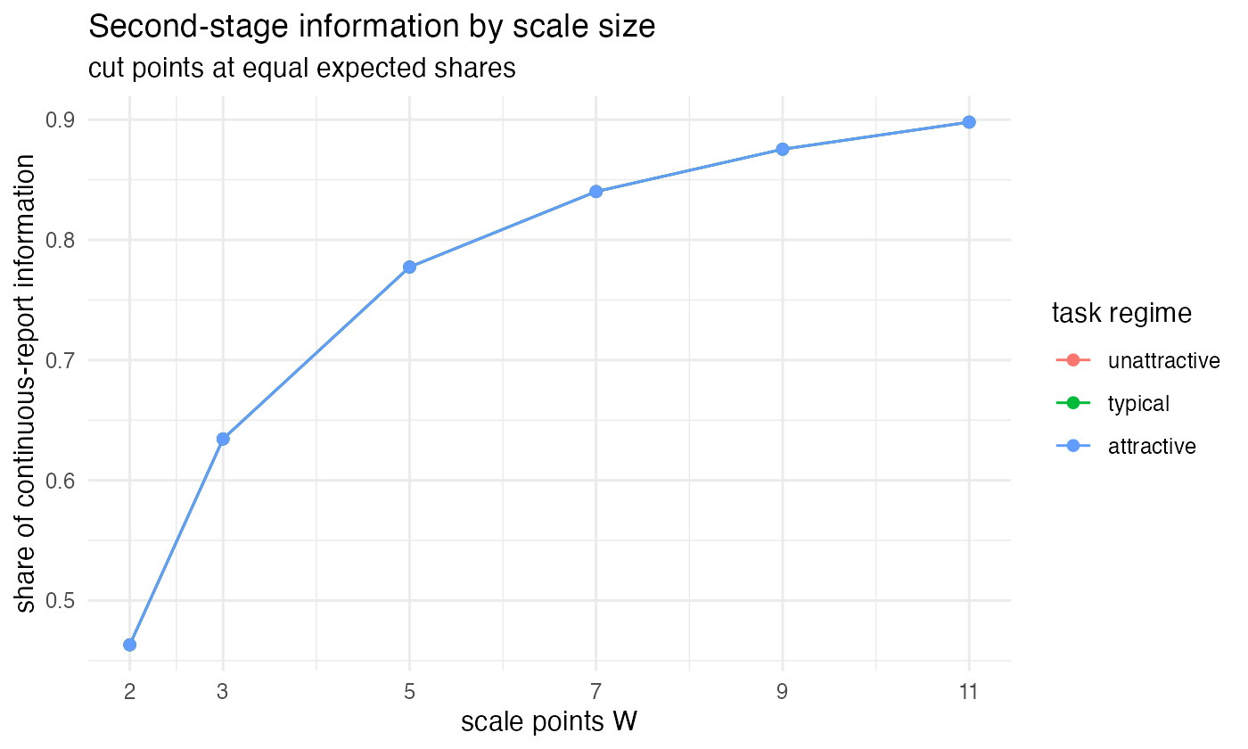
Notebook 7 turns the information results of Section 2.8 into design guidance (Figure 3). With cut points at equal expected shares, a binary follow-up captures 46% of the continuous-report information limit and five points capture 78%; the increment beyond seven points is small. Cut placement matters as much as cut count: information-optimal cuts recover a further 15% over equal-share placement, and label sets that produce the skewed usage typical of fielded purchase-intent scales cost 29% relative to optimal.
3.7 Economic Stakes: A Pricing Counterfactual
Finally, notebook 8 asks what each estimator implies for pricing. A synthetic market of five brands with a quality attribute, wide price variation, and heterogeneous preferences calibrated to own-price elasticities of about -1.9 generates \(W = 5\) dual-response data (\(N = 500\), \(T = 12\)); each estimator’s demand system then sets Nash equilibrium prices by damped best responses, verified from multiple starts. All systems define demand the same way, as top-2-box purchase, so a binary estimator dichotomized at that threshold answers the question it was fit to. Posterior-predictive demand uses full parameter draws rather than posterior means, which would flatten heterogeneity.
| estimator | mean |price err| % | max |price err| % | profit forecast err % | profit forgone % |
|---|---|---|---|---|
| ordinal | 1.11 | 2.13 | -2.98 | 0.37 |
| bin_t2b | 1.10 | 2.38 | -2.47 | -0.31 |
| bin_top | 2.57 | 5.73 | -59.29 | -0.84 |
| heur_juster | 4.84 | 8.52 | 105.82 | 2.18 |
| heur_t2b | 4.84 | 8.52 | 52.94 | 2.18 |
In Table 3, the full ordinal model prices the market almost exactly. The well-placed binary dual response also prices well, consistent with the efficiency analysis, but the analyst does not get to choose the placement after the fact: dichotomizing at the top box misprices by up to 5.7% and misstates its own profit forecast by 59%, because a top-box model can only answer a top-box question. The constant-probability heuristic fails for a different reason. Its purchase incidence cannot respond to price, so it underprices systematically: the calibration constant cancels from every best response, and its equilibrium is the inside-good-only equilibrium. It also overstates forecast profits by 106%. Because the constant itself causes the failure, no choice of constant and no amount of data repairs it.
4 Empirical Application
We illustrate the model with data from a commercial choice-based conjoint study conducted in partnership with a consumer insights consultancy, in which an ordinal purchase-likelihood question followed each choice task.
4.1 Data
4.2 Model Specifications and Estimation
We estimate four specifications on the same data: our model (Section 2) in aggregate and hierarchical form; the binary dual-response benchmark applied to the dichotomized scale (top-2-box); and the constant-probability heuristic. Hierarchical specifications use the sampler of Section 2.10.
Pre-specified test battery. Before any model comparison, we commit to the three specification tests of Section 2.7 on the aggregate fit: the unit-slope test (\(\lambda = 1\)), the conditioning test (\(\delta = 0\)), and the DR-2Max test (\(\delta = 1\)), whose operating characteristics Section 3.4 establishes, together with a test, by holdout likelihood and WAIC, of our model’s complementary log-log link against the logit link of the resolved comparison. We also commit to re-running the pricing counterfactual of Section 3.7 on the empirical posteriors, replacing the synthetic market with the study’s own category structure.
4.3 Results
4.4 Scale-Usage Heterogeneity
5 Discussion
5.1 What the Behavioral Model Changes
The premise that the consumer observes everything about the inside goods but not the outside-good shock also changes how the dual-response literature’s models relate to one another. In the binary literature, the choice between DR-2Max and DR-AnyMax was framed as a matter of how the second question is worded, that is, whether the consumer evaluates her selected option or the whole set (Diener et al. 2006), and the shared-error Unified Model of Hung, Liu, et al. (2025) was motivated by the internal consistency of a single utility draw. Our framework arrives at the inclusive-value form from the primitive assumption about information: because the maximum of Gumbel utilities is independent of which good attains it, any coherent report about the best option’s standing against the outside good must depend on the task only through its inclusive value. The empirical success of the AnyMax/Unified form over DR-2Max, documented in both Diener et al. (2006) and Hung, Liu, et al. (2025), is what our framework predicts. Where our account differs from Brazell et al. (2006) is in what the second response is. They treat it as a second choice from an augmented set; we treat it as a report about an unresolved comparison, and that reading is what licenses asking for it on an ordinal scale.
The choice of link encodes a behavioral assumption about when the consumer resolves the outside-good shock. For a binary follow-up both accounts are coherent and they disagree: resolving the outside-good draw first recovers the standard logit second stage, while our model implies a complementary log-log one even for yes/no data. Because the two diverge mainly in the tails, telling them apart requires either large samples or designs with wide variation in task attractiveness. Section 4 provides evidence from one commercial dataset; we regard the question as open and worth testing on the many existing binary dual-response datasets, where our model’s binary case can be estimated with a one-line change to current code. For an ordinal follow-up the question does not arise in the same form, since a consumer who has resolved the outside good holds no graded likelihood to report.
5.2 Implications for Practice
Four points bear directly on applied work. First, if an ordinal dual response has been fielded, dichotomizing it is costly and arbitrary: the analyst chooses the cut before seeing the data, the penalty ranges from a few percent of sample at a lucky cut to a third of it at an unlucky one (Section 3.3), the damage concentrates at the individual level where hierarchical estimation lives, and a dichotomized model can answer questions only at its own threshold; the pricing counterfactual’s top-box analyst misstates the profit forecast by more than half for that reason. Second, constant-probability weighting fails at any sample size. Beyond the set-dependence of scale-point meaning (Equation 8 and Table 6), a fixed purchase incidence cancels out of every pricing first-order condition, so the heuristic’s price recommendations ignore the no-buy margin. Third, the information results in Section 2.8 and Section 3.6 give concrete design guidance: five scale points capture most of the binary-to-continuous information gap (about 78%, versus 46% for binary), gains beyond seven points are small, and where the labels place the cut points matters as much as how many there are. Fourth, studies that intend to test the behavioral model (the link, the unit slope) should engineer variation in task attractiveness; designs without it cannot discriminate the links even in principle (Section 2.6). Notebook 7 confirms the point with a design that shifts each task’s prices until every task has the same inclusive value: the design still identifies \(\bfbeta\), but it no longer tells the links apart.
5.3 Relation to the Outside-Good Literature
Our model holds the outside good’s mean utility fixed at zero and locates all action in the consumer’s uncertainty about its realization. Two adjacent strands suggest natural extensions. Hung, Liu, et al. (2025) show that a budget constraint applied to the second response, but not to the forced choice, improves fit and materially changes equilibrium price predictions; the same asymmetric treatment is available here, censoring the ordinal report for options priced above a consumer-level budget, and the ordinal response should sharpen identification of the budget, since near-threshold options will earn lukewarm rather than merely negative reports. Hung, Kurz, et al. (2025) document that the no-choice option’s utility can drift over the course of a survey as consumers learn about the category; in our notation the drift is in the cut points (or in the outside-good location), and the task-order diagnostics of Section 4.1 carry over directly. More broadly, the opt-out literature’s warning that a single constant rarely captures heterogeneous non-purchase behavior (Campbell and Erdem 2019; Haaijer et al. 2001) applies to the dual response as well; the heterogeneous-cut-point extension of Section 2.9.1 is one response, and richer structures (e.g., serial non-purchasers as a latent class) are compatible with the framework.
5.4 Limitations
Five limitations qualify the results. First, the results depend on the Gumbel error assumption: the factorization of the joint likelihood and the inclusive-value form of the second response both rest on max-stability. Appendix D shows how far the assumption can be relaxed. Any generalized extreme value structure, nested logit included, preserves both properties once the inclusive value is redefined as the GEV generator, so correlation among the displayed alternatives costs the framework nothing. Error families outside that class do break the closed form: under a probit or a mixed logit with a correlated kernel the max utility has no closed-form distribution, and the second response would require simulation over it. Our robustness experiments soften the concern in one direction: with variance-matched normal errors, preference and demand estimates are essentially unimpaired because the cut points absorb the misspecification, so the cut points deserve more caution as structural parameters than do the demand quantities built from them. Second, we treat tasks as independent draws, abstracting from learning, fatigue, and reference formation across the sequence (Hung, Kurz, et al. 2025); the task-order diagnostic of Section 3.5 detects such drift reliably when present. Third, the common-cut-point model assumes a shared reading of the scale labels; the extension of Section 2.9.1 relaxes the assumption, but individual-level identification is thin at commercial task counts, and our simulations find that ignoring moderate scale-usage heterogeneity costs little, so the extension is most useful as a diagnostic and as insurance. Fourth, like all stated-preference methods, the model calibrates stated rather than revealed purchase behavior; the ordinal report inherits whatever hypothetical bias attends purchase-intent questions generally (Morrison 1979), though Wlömert and Eggers (2016), recontacting respondents five months after a service launch, find that the binary dual response improves predictive accuracy against realized adoption, and linking the estimated cut points to realized purchase rates (the ordinal analogue of the calibration literature on binary intentions) is a natural next step. Fifth, the likelihood presumes the two questions are asked together, as in the standard dual-response task. Designs that separate them, such as the separated dual response of Schlereth and Skiera (2017), break the coupling between the two responses and would require modeling the stages as separate draws. Appendix C documents a separate methodological caution: harmonic-mean estimates of the marginal likelihood are optimistic, so we anchor model comparisons in holdout likelihood and WAIC alongside the conventional estimator.
6 Conclusion
Dual-response conjoint separates a question consumers answer readily, which of these do you like best, from one they cannot answer with certainty, would you actually buy it. This paper takes that uncertainty as the modeling primitive. A consumer who observes everything about the displayed alternatives but not her valuation of the outside good holds a purchase probability rather than a decision, so the natural follow-up question is ordinal and the natural model joins a multinomial logit for the forced choice to a cumulative-link ordinal model on the task’s inclusive value. The link function is not a modeling choice. It follows from whether the consumer reports the probability she still holds, as our model has her do, or resolves her uncertainty and grades the comparison that results, and the two are distinguishable on data that vary the attractiveness of the displayed alternatives.
At two scale points the logistic link is the incumbent binary dual-response model, so the ordinal form extends that literature and contains its leading model. Our model’s binary case, however, is a complementary log-log response, so the familiar yes/no follow-up is mildly misspecified, a claim that data already collected can test. A finer scale never subtracts information, and five points capture most of the gap between a binary answer and a continuous one. The two ways an ordinal report is otherwise reduced to something the binary model accepts both fail: collapsing the scale at an arbitrary point wastes information, and assigning each point a fixed purchase probability is internally inconsistent, because the meaning of a scale label depends on what was on the screen. Simulation evidence confirms that the aggregate and hierarchical Bayesian estimators recover the model’s parameters, including the cut points that give the scale labels quantitative meaning, and that the conclusions survive correlated alternatives, non-Gumbel errors, and drift in the outside good across a consumer’s task sequence.
A finer response scale is worth fielding only if the analysis can use the extra categories. The likelihood derived here uses all of them, and it opens further work on calibrating estimated cut points against realized purchase behavior, on using the ordinal response to identify budget constraints, and on the design of the scale itself.
Appendix A: Proofs
A.1 Proof of Lemma 1
The result is classical (McFadden 1981). We give the derivation because part (ii) carries Equation 10, and because Appendix D extends this calculation to generalized extreme value errors.
Let \(u_j = V_j + \eta_j\) with \(\eta_j \iid \text{Gumbel}(0,1)\) for \(j \in \mathcal{J}^+\), so \(u_j\) has CDF \(F_j(t) = \exp\left( -e^{-(t - V_j)} \right)\) and density \(f_j(t) = e^{-(t-V_j)} \exp\left( -e^{-(t-V_j)} \right)\). For any \(j\) and any \(u\), \[ \Pr \left( j^* = j, \; u^* \le u \right) = \int_{-\infty}^{u} f_j(t) \prod_{k \ne j} F_k(t) \, dt = \int_{-\infty}^{u} e^{V_j} e^{-t} \exp \left( -e^{-t} S \right) dt, \] using \(\prod_{k \ne j} F_k(t) = \exp\left( -e^{-t} \left( S - e^{V_j} \right) \right)\) with \(S = \sum_{k} e^{V_k}\), and collecting terms. Substituting \(s = e^{-t} S\) (so \(ds = -e^{-t} S \, dt\)) gives \[ \Pr \left( j^* = j, \; u^* \le u \right) = \frac{e^{V_j}}{S} \int_{e^{-u} S}^{\infty} e^{-s} \, ds = \underbrace{\frac{e^{V_j}}{S}}_{\Pr\left(j^*=j\right)} \; \times \; \underbrace{\exp \left( -S e^{-u} \right)}_{F_{\text{Gumbel}\left(\overline{\mu},1\right)}(u)}. \] Letting \(u \to \infty\) delivers the MNL choice probability; summing over \(j\) delivers \(u^* \sim \text{Gumbel}(\overline{\mu}, 1)\) with \(\overline{\mu} = \ln S\); and the factorization of the joint law for every \((j, u)\) is the independence of \(j^*\) and \(u^*\). \(\square\)
The calculation is short but gives little sense of why the two quantities separate. A change of variable makes the reason transparent, and the same argument extends to correlated alternatives in Appendix D.
Write \(y_j = e^{V_j}\) and set \(T_j = e^{-u_j}\). The map is decreasing, so it exchanges maxima for minima: the best good is the one with the smallest \(T_j\), and \(u^* = -\ln \min_j T_j\). Under the Gumbel assumption, \[ \Pr \left( T_j > t \right) = \Pr \left( u_j < -\ln t \right) = e^{-y_j t}, \] so each good becomes an independent waiting time that arrives at the constant rate \(y_j\), and the consumer’s chosen good is whichever arrives first.
For independent waiting times of this kind, the identity of the first arrival and the time of that arrival are independent, because the rates do not change as time passes. At any instant, given that nothing has yet arrived, the chance that the next arrival is good \(j\) is \(y_j / S\), the same at the start as at any later point. Which good arrives first is therefore settled entirely by the rates relative to one another, while how long the wait lasts is settled entirely by their sum \(S\). Waiting longer says nothing about who will win. Transforming back, the shares \(y_j / S\) are the multinomial logit probabilities and the total \(S\) fixes the location of \(u^*\), which is the content of Lemma 1. This is the division of labor between the two responses. The rates relative to one another are the utility differences that the forced choice reveals, and their sum is the inclusive value that the ordinal report reads, so the two responses read separate features of the same draw.
The same statement in utility terms is that the relative odds of being the maximizer are the same at every level of the maximum, because Gumbel upper tails decay exponentially and are therefore shift-invariant: \(\Pr(u_1 > m) / \Pr(u_2 > m) = e^{V_1 - V_2}\) for every \(m\).
The property belongs to the extreme-value family, not to random utility models in general. Under normal errors with \(V_1 > V_2\), the ratio of upper tails diverges as \(m\) grows, so a high realized maximum is disproportionately likely to have come from the better alternative. The level of the maximum then carries information about which alternative attained it, the joint law of \(\left( j^*, u^* \right)\) does not factor, and the counterpart of Equation 10 is unavailable. Appendix D shows that the factorization survives correlation among the inside goods, because the waiting times may be dependent and still arrive at rates whose ratios are constant over time; what fails outside the extreme-value family is the constancy of those ratios.
A.2 Derivation of the information increment (Equation 16)
The second response contributes the multinomial log-likelihood \(\ell = \sum_w \mathbb{1}\lbrace y = w \rbrace \ln \pi_w\) with \(\pi_w = F(c_w - \overline{\mu}) - F(c_{w-1} - \overline{\mu})\). Since \(\partial \overline{\mu} / \partial \bfbeta = \sum_j \Pr(j^* = j) \, \x_j = \overline{\x}\), the score with respect to \(\bfbeta\) in category \(w\) is \(- \left[ f_w - f_{w-1} \right] / \pi_w \cdot \overline{\x}\), writing \(f_w = f \left( c_w - \overline{\mu} \right)\) and \(f = F'\) (with \(f_0 = f_W = 0\)). The information is the expected outer product of the score: \[ \mathcal{I}^{(2)} = \sum_{w=1}^{W} \pi_w \left( \frac{f_w - f_{w-1}}{\pi_w} \right)^2 \overline{\x} \, \overline{\x}' = \left[ \sum_{w=1}^{W} \frac{ \left( f_w - f_{w-1} \right)^2 }{ \pi_w } \right] \overline{\x} \, \overline{\x}' = \omega \left( \overline{\mu}; \mathbf{c} \right) \overline{\x} \, \overline{\x}'. \qquad \square \] The joint information over \(\left( \bfbeta, \mathbf{c} \right)\), including the cut-point blocks used by the estimation code, follows from the same score with \(\partial \pi_w / \partial c_m = f_w \mathbb{1}\lbrace m = w \rbrace - f_{w-1} \mathbb{1}\lbrace m = w-1 \rbrace\).
A.3 Monotonicity of \(\omega\) under refinement
Let \(\mathcal{C}'\) be a coarsening of the partition \(\mathcal{C}\) obtained by merging adjacent categories \(w\) and \(w+1\). The merged cell contributes \(\left( f_{w+1} - f_{w-1} \right)^2 / \left( \pi_w + \pi_{w+1} \right)\) to \(\omega'\), while the two original cells contribute \(\left( f_w - f_{w-1} \right)^2 / \pi_w + \left( f_{w+1} - f_w \right)^2 / \pi_{w+1}\) to \(\omega\). Writing \(a = f_w - f_{w-1}\), \(b = f_{w+1} - f_w\), \(u = \pi_w\), \(v = \pi_{w+1}\), the Cauchy–Schwarz inequality in Engel form gives \[ \frac{(a + b)^2}{u + v} \;\le\; \frac{a^2}{u} + \frac{b^2}{v}, \] so each merge weakly decreases \(\omega\), and so does any coarsening, which is a finite sequence of adjacent merges. The binary response is the coarsest member of the family and hence the least informative; conversely, as the mesh of the partition goes to zero the interval score converges to the exact-observation score and \(\omega \to \int \left( g' \right)^2 / g \, dz\), the Fisher information of the latent variable’s location (equal to \(1\) for the standard Gumbel and \(1/3\) for the standard logistic). \(\square\)
A.4 The purchase probability is \(\text{Beta}(S,1)\)
From the researcher’s perspective the consumer’s purchase probability \(p_{it} = F \left( u^*_{it} \right)\) is a random variable, and its distribution is Beta with the inclusive value as its only shape parameter. The ingredients are classical: the max-stability of the Gumbel family (McFadden 1981) and the probability integral transform.
Drop subscripts and write \(F(z) = \exp \left( -e^{-z} \right)\) for the standard Gumbel CDF and \(F_{\overline{\mu}}\) for the \(\text{Gumbel}(\overline{\mu},1)\) CDF. Max-stability is the statement that shifting the location is the same as raising the CDF to a power: \[ F_{\overline{\mu}}(z) = \exp \left( -e^{-(z - \overline{\mu})} \right) = \exp \left( -e^{-z} e^{\overline{\mu}} \right) = \left[ \exp \left( -e^{-z} \right) \right]^{S} = F(z)^{S}, \qquad S = e^{\overline{\mu}}. \] By Lemma 1(i), \(u^* \sim \text{Gumbel}(\overline{\mu},1)\), and \(F\) is strictly increasing, so for \(a \in (0,1)\) \[ \Pr \left( p \le a \right) = \Pr \left( F(u^*) \le a \right) = \Pr \left( u^* \le F^{-1}(a) \right) = F_{\overline{\mu}} \left( F^{-1}(a) \right) = F \left( F^{-1}(a) \right)^{S} = a^{S}. \] The explicit form of \(F^{-1}\) is never needed; the last step is \(F(F^{-1}(a)) = a\). Differentiating gives the density \(S a^{S-1}\) on \([0,1]\). The \(\text{Beta}(\alpha, \beta)\) density is \(a^{\alpha-1} (1-a)^{\beta-1} / B(\alpha,\beta)\), and at \((\alpha,\beta) = (S,1)\) the factor \((1-a)^{\beta-1}\) is one while \(B(S,1) = \Gamma(S)\Gamma(1) / \Gamma(S+1) = 1/S\), so the two densities coincide: \(p \sim \text{Beta}(S,1)\). The mean follows as \(\E[p] = S / (S+1) = \Lambda(\overline{\mu})\). \(\square\)
Reading \(S\) as a count. For integer \(S\), max-stability says that \(\text{Gumbel}(\ln S, 1)\) is the distribution of the maximum of \(S\) iid standard Gumbel draws, and the probability integral transform makes each \(F(\eta_k)\) a standard uniform. Since \(F\) is increasing it passes through the maximum, so \[ p = F \left( \max_{k \le S} \eta_k \right) = \max_{k \le S} F \left( \eta_k \right) = \max_{k \le S} U_k, \qquad U_k \iid \text{Uniform}(0,1), \] and the maximum of \(S\) iid uniforms is \(\text{Beta}(S,1)\) by the usual order-statistic calculation. The consumer’s purchase probability therefore behaves like the best of \(S\) independent uniform draws, which is the sense in which \(S_{it} = e^{\overline{\mu}_{it}}\) measures how many chances the choice set gets. The reading is heuristic, since \(S_{it} = \sum_j e^{V_{itj}}\) is not generally an integer, but the distribution above holds for every real \(S > 0\).
Appendix B: Estimation Details
Aggregate model. We maximize the likelihood over the working parameters \(\left( \bfbeta, c_1, \ln(c_2 - c_1), \ldots, \ln(c_{W-1} - c_{W-2}) \right)\), which enforce cut-point monotonicity without constraints; standard errors for the cut points follow by the delta method. We compute interval probabilities with tail-stable expressions (\(\Lambda(h)\Lambda(-l)(1 - e^{l-h})\) for the logistic link and \(e^{-e^{-h}}\left(1 - e^{-(e^{-l} - e^{-h})}\right)\) for the Gumbel link) so that extreme cut points do not lose precision to cancellation.
Hierarchical model. The sampler is a random-walk Metropolis-within-Gibbs in the style of Rossi et al. (2005) with three blocks per iteration: (1) all consumers’ \(\bfbeta_i\) (and, in the heterogeneous-cut-point extension, \(\bftheta_i\)) are updated simultaneously by independent normal random-walk proposals with covariance \(s_i^2 \Sigma\); (2) the common cut-point block is updated by a random-walk proposal on the unconstrained scale; (3) the population moments \(\left( \betabar, \Sigma \right)\) are drawn from their conjugate normal and inverse-Wishart conditionals. Priors: \(\betabar \sim \mathcal{N}\left( \mathbf{0}, 100 I \right)\), \(\Sigma \sim \text{IW}\left( \dim + 3, (\dim + 3) I \right)\), and \(\mathcal{N}(0, 100 I)\) on the transformed cut points. Step sizes are initialized at \(2.93/\sqrt{\dim}\) and adapted only during burn-in toward acceptance rates of \(0.23\) (individual blocks) and \(0.30\) (cut-point block). Unless noted, we run 30,000 iterations, discard 10,000, and keep every 10th draw.
We validated the sampler four ways (replication code accompanies the paper): parameter recovery on synthetic panels for both links; repeated-sampling coverage of 50% and 90% posterior intervals at nominal rates; agreement of the forced-choice-only special case with an independent hierarchical-MNL implementation (posterior means matching to less than 0.01 on all hyperparameters on common data); and convergence of the posterior toward the aggregate MLE when the data are generated without heterogeneity.
Appendix C: Marginal-Likelihood Estimation
Model comparisons in the paper report the log marginal density (LMD). For hierarchical models we follow the standard practice in this literature (Hung, Liu, et al. 2025) and use the harmonic-mean estimator of Newton and Raftery (1994), complemented by two quantities that do not rely on it: the WAIC computed from pointwise per-consumer likelihoods (Watanabe 2010; Vehtari et al. 2017) and the log posterior-predictive density of held-out tasks. We add them because the harmonic-mean estimator is optimistic. In the aggregate model, where the parameter space is small enough for exact methods, we can measure the bias directly: bridge sampling (Meng and Wong 1996; Gronau et al. 2020) and a Laplace approximation agree with each other to well under one log point, while the Newton–Raftery estimate exceeds them by dozens of log points, and trimming the smallest-likelihood draws widens rather than closes the gap:
| estimator | log marginal density | vs. bridge |
|---|---|---|
| bridge | -9844.14 | 0.00 |
| laplace | -9844.15 | -0.01 |
| NR | -9801.78 | 42.36 |
| NR trim 5% | -9799.63 | 44.51 |
| NR trim 20% | -9798.42 | 45.73 |
Because the bias is similar for models of similar dimension, Newton–Raftery rankings between the ordinal and binary dual-response models are typically preserved, but we treat the WAIC and holdout comparisons as primary whenever the two disagree.
Appendix D: Correlated Alternatives
Lemma 1 is stated for independent Gumbel errors, and the whole of Section 2 rests on it. Both of its properties hold for the entire generalized extreme value (GEV) family of McFadden (1981), so that correlation among the inside goods costs the framework nothing beyond a redefinition of the inclusive value.
Let the inside-good components have the GEV joint distribution \[ \Pr \left( \eta_1 \le e_1, \ldots, \eta_J \le e_J \right) = \exp \left( - G \left( e^{-e_1}, \ldots, e^{-e_J} \right) \right), \tag{19}\] where the generator \(G : \mathbb{R}^J_{+} \to \mathbb{R}_{+}\) is homogeneous of degree one, tends to infinity in each argument, and has mixed partial derivatives that alternate in sign. Independent Gumbel errors are the special case \(G(y) = \sum_j y_j\). Write \(y_j = \exp(V_j)\), \(G_j = \partial G / \partial y_j\), and \[ S^{G} \coloneqq G \left( y_1, \ldots, y_J \right), \qquad \overline{\mu} \coloneqq \ln S^{G}. \tag{20}\]
Lemma 2 Under Equation 19, with \(u_j = V_j + \eta_j\) and \(u^* = \max_{j} u_j\):
\(u^* \sim \text{Gumbel} \left( \overline{\mu}, 1 \right)\) with \(\overline{\mu} = \ln S^{G}\);
\(j^*\) and \(u^*\) are statistically independent, with \(\Pr(j^* = j) = y_j G_j(y) / S^{G}\).
Proof. The joint CDF of the utilities is \[ H \left( m_1, \ldots, m_J \right) = \exp \left( - G \left( y_1 e^{-m_1}, \ldots, y_J e^{-m_J} \right) \right). \] For (i), set every \(m_j = m\) and use homogeneity of degree one: \(G(y e^{-m}) = e^{-m} G(y)\), so \(H(m, \ldots, m) = \exp \left( - e^{-m} S^{G} \right)\), which is the \(\text{Gumbel}\left(\ln S^{G}, 1\right)\) CDF.
For (ii), write \(t_k = y_k e^{-m_k}\) and differentiate: \[ \frac{\partial H}{\partial m_j} = \exp \left( -G(t) \right) \, G_j(t) \, y_j e^{-m_j}. \] Because \(G\) is homogeneous of degree one, \(G_j\) is homogeneous of degree zero, so evaluating at \(m_k = s\) for every \(k\) gives \(G_j(t) = G_j(y)\) and \(G(t) = e^{-s} S^{G}\). Hence \[ \left. \frac{\partial H}{\partial m_j} \right|_{m_k = s \ \forall k} = \exp \left( - e^{-s} S^{G} \right) G_j(y) \, y_j e^{-s} = \frac{y_j G_j(y)}{S^{G}} \cdot \frac{d}{ds} \exp \left( - e^{-s} S^{G} \right), \] and integrating from \(-\infty\) to \(u\), \[ \Pr \left( j^* = j, \ u^* \le u \right) = \underbrace{\frac{y_j G_j(y)}{S^{G}}}_{\Pr \left( j^* = j \right)} \; \times \; \underbrace{\exp \left( - e^{-u} S^{G} \right)}_{\Pr \left( u^* \le u \right)} \] for every \(j\) and every \(u\), which is the claimed independence. Letting \(u \to \infty\) recovers the GEV choice probability. \(\square\)
Everything in Section 2 follows with \(S_{it}\) replaced by \(S^{G}_{it}\). The first response becomes the GEV choice probability rather than the multinomial logit; the second response is unchanged in form, since Equation 7, Equation 12, and the cumulative-link representation Equation 9 depend on the choice set only through \(\overline{\mu}_{it}\); and the factorization Equation 10 holds for the same reason as before. The location invariance behind Proposition 1 also survives: shifting every \(V_{itj}\) by \(\delta\) multiplies \(S^{G}_{it}\) by \(e^{\delta}\) and so shifts \(\overline{\mu}_{it}\) by exactly \(\delta\), which the cut points absorb. The rank condition must then be read against the design as it enters \(G\) rather than a simple sum, and the nesting result of Section 2.5 becomes \(\Pr(\text{buy}) = S^{G}_{it} / \left( e^{\gamma} + S^{G}_{it} \right)\).
The leading application is nested logit, \(G(y) = \sum_{n} \left( \sum_{j \in n} y_j^{1/\lambda_n} \right)^{\lambda_n}\), in which alternatives within a nest are correlated whenever \(\lambda_n < 1\). We confirm Lemma 2 numerically for a five-alternative, two-nest design with \(\lambda = (0.5, 0.8)\) using the positive-stable mixture representation of the nested logit (R/homogeneous/gev_check.R). Across two million draws the simulated distribution of \(u^*\) matches \(\text{Gumbel}(\ln S^{G}, 1)\) (location \(1.845\) against \(1.846\) analytically; Kolmogorov–Smirnov \(p = 0.17\)), the simulated choice shares match \(y_j G_j / S^{G}\) to four decimal places, and the conditional distribution of \(u^*\) given \(j^*\) is indistinguishable from its unconditional counterpart at every quartile (chi-square test of independence, \(p = 0.70\)).
The result has two limits. It covers correlation among the inside goods only: the outside-good shock \(\eta_{it0}\) is assumed independent of them throughout, and the logistic link uses that independence to obtain \(d_{it} \sim \text{Logistic}(\overline{\mu}_{it}, 1)\). And it does not extend to error structures outside the GEV class, such as multinomial probit or a mixed logit with correlated kernel errors, for which \(u^*\) has no closed-form distribution and the factorization that makes Equation 10 tractable is unavailable.
Appendix E: Implementation in Apollo
The replication archive implements the model twice: once directly, in the routines described in Appendix B, and once in Apollo (Hess and Palma 2019), the freeware choice-modeling package for R. The second implementation serves two purposes. It cross-validates our code against an independently developed and widely used toolkit, and it shows how the model fits into an estimation framework readers may already have installed.
The model as a two-component structure. Apollo builds a likelihood by multiplying components. Our joint likelihood Equation 10 has that form, so the forced choice is an apollo_mnl component and the ordinal follow-up is a second component over the same tasks. Hybrid choice models, a common use of the package, share this architecture: they combine a multinomial logit for the choice with ordered-response components for attitudinal indicators (Daly et al. 2012). The difference between the two is the content of Section 2. In a hybrid choice model the ordinal component is driven by a latent attitude that is exogenous to the choice, and it is connected to the choice utilities through freely estimated loading parameters. Here the ordinal component is driven by the inclusive value of the same choice set, and its loading is fixed at one rather than estimated. Our model is the restricted case, and Lemma 1 justifies the restriction.
The logistic specification is native; ours is not. With the second stage a cumulative logit in \(\overline{\mu}_{it}\), the logistic specification is assembled from stock parts: apollo_mnl for the choice, apollo_ol for the follow-up with the task’s inclusive value passed as its single explanatory variable and the cut points as its thresholds, and apollo_combineModels to join them. Our model has no stock part. Apollo supplies ordered components for the logistic and normal links and no others, so the complementary-log-log form Equation 7 must be written out and passed through apollo_ownModel, the hook for user-defined likelihoods. The function is short, and once supplied it inherits the rest of the package. The asymmetry also shows that the standard toolkit anticipates the behavior in which the consumer resolves her uncertainty before answering, and not the behavior in which she reports the probability she still holds.
Agreement. Table 5 reports the largest discrepancy between the two implementations over 5 independent datasets of 2,000 tasks in each of two configurations, with both implementations started from the same values.
| configuration | ordinal component | beta | cut points | standard errors | log-likelihood |
|---|---|---|---|---|---|
| Our model, W = 5 | apollo_ownModel | 1e-06 | 2e-06 | 1e-07 | 9e-10 |
| Logistic, W = 2 (binary) | apollo_ol | 5e-07 | 5e-07 | 5e-09 | 6e-11 |
Point estimates agree to 2e-06 or better, standard errors to 1e-06, and the maximized log-likelihood to 9e-10, which is convergence tolerance rather than disagreement. The two implementations share no code: Apollo computes the ordinal probabilities for our model from the direct expression \(e^{-e^{-(c_w - \overline{\mu})}} - e^{-e^{-(c_{w-1} - \overline{\mu})}}\), while ours uses the tail-stable rearrangement of Appendix B, and the cut points enter Apollo’s likelihood as free parameters rather than through the monotone increment parameterization. The binary row is the incumbent dual-response model of Diener et al. (2006) and Hung, Liu, et al. (2025), recovered as the two-point special case of Section 2.5.
Why the hierarchical model is not estimated in Apollo. Apollo reaches Bayesian estimation by wrapping RSGHB, which requires each random parameter to be assigned one of a fixed menu of marginal distributions: normal, log-normal, censored normal, or Johnson SB. None of them can express an ordered vector. The heterogeneous-cut-point extension of Section 2.9.1 gives each consumer her own thresholds \(\bftheta_i\), which must stay ordered for the likelihood to be defined, and we impose that through a transformation to an unconstrained scale inside a random-walk block. A purpose-written sampler can express that; the RSGHB menu cannot. The restriction is specific to the Bayesian path: apollo_ol accepts thresholds that vary across observations, so classical mixed-threshold specifications are available. The hierarchical results in Section 3 therefore come from the sampler of Appendix B rather than from Apollo.
Appendix F: The Model in Miniature
The smallest interesting instance of the model makes the machinery concrete: two consumers with identical preferences, one attribute, one task each, and a three-point scale.
Let both consumers share the scalar taste parameter \(\beta = 1\), which we treat as known for the arithmetic. Each faces one task with two inside goods described by a single attribute \(x\), answers the forced choice, and then reports on the three-point scale \(\mathcal{W} = \lbrace \text{"unlikely"}, \text{"unsure"}, \text{"likely"} \rbrace\) with utility-scale cut points \(\mathbf{c} = (c_1, c_2) = (0, 2)\). (In our model these correspond to probability-scale cut points \(\left( \alpha_1, \alpha_2 \right) = \left( F(0), F(2) \right) = (0.37, 0.87)\): the consumer answers “unsure” when her purchase probability lies between 37% and 87%.) The two tasks, one for each consumer, differ in the level of the attribute but not in its spread: consumer 1 faces an attractive pair, \(x = (2, 1)\), and consumer 2 an unattractive pair, \(x = (-1, -2)\).
Consider the model’s account of their behavior, giving both consumers the same realized components \(\eta = (0.30, -0.86)\) on their two inside goods. Consumer 1’s utilities are \(u = (2.30, 0.14)\): she picks her first good and knows her best utility, \(u^* = 2.30\). She cannot resolve the outside-good shock \(\eta_0\), so she reports the bin containing her purchase probability \(p = F(2.30) = 0.90\), namely “likely.” Consumer 2’s utilities are \(u = (-0.70, -2.86)\): she also picks her first good, but her best utility is \(u^* = -0.70\), her purchase probability is \(F(-0.70) = 0.13\), and she reports “unlikely.” The two consumers made identical first-response choices from identical realizations, yet gave opposite second responses.
The walkthrough fixed one set of draws. Averaging over all of them, as the researcher must, shows that the pattern does not depend on that draw (Table 6). The forced-choice probabilities are the same function of the data for both consumers: the MNL depends only on the within-task difference \(x_1 - x_2 = 1\), so \(\Pr(\text{choose better good}) = \Lambda(\beta) = 0.73\) in both tasks. The forced choice reveals how much she prefers one option to the other, but nothing about how much she wants either. The tasks separate only through the inclusive value (\(S_1 = e^2 + e^1 = 10.11\) versus \(S_2 = e^{-1} + e^{-2} = 0.50\), i.e., \(\overline{\mu}_1 = 2.31\) versus \(\overline{\mu}_2 = -0.69\)), which the cumulative-link stage compares against the cut points. (With \(c_1 = 0\), consumer 2’s probability of “unlikely” is \(\Lambda(-\overline{\mu}_2) = 1/(1+S_2) = 0.67\), the familiar no-choice probability of the single-stage MNL, which previews the nesting results below.)
| Consumer 1 (attractive task) | Consumer 2 (unattractive task) | |
|---|---|---|
| Attribute values \(x\) | \((2,\ 1)\) | \((-1,\ -2)\) |
| \(\Pr(\text{choose better good})\) | \(0.73\) | \(0.73\) |
| \(S = \sum_j e^{V_j}\), \(\ \overline{\mu} = \ln S\) | \(10.11\), \(\ 2.31\) | \(0.50\), \(\ -0.69\) |
| \(\Pr(y = w)\) | \((0.00,\ 0.25,\ 0.75)\) | \((0.60,\ 0.33,\ 0.07)\) |
| \(\E \left[ p \mid y = \text{"unsure"} \right]\) | \(0.80\) | \(0.60\) |
The joint likelihood of the observed data, in which each consumer chose her better good and \(y_1 = \text{"likely"}\), \(y_2 = \text{"unlikely"}\), follows from Equation 10: \[ L \left( \beta, \alpha_1, \alpha_2 \right) = \underbrace{\Lambda(\beta) \Big[ 1 - \alpha_2^{\,S_1(\beta)} \Big]}_{\text{consumer 1:} \ \ 0.73 \times 0.75} \times \underbrace{\Lambda(\beta) \, \alpha_1^{\,S_2(\beta)}}_{\text{consumer 2:} \ \ 0.73 \times 0.60}, \tag{21}\] with \(S_1(\beta) = e^{\beta} \left( 1 + e^{\beta} \right)\) and \(S_2(\beta) = e^{-2\beta} \left( 1 + e^{\beta} \right)\). Two general points follow from the example.
First, the two responses divide the labor of identification, a division that Proposition 1 formalizes. The forced-choice factors involve only utility differences, and they identify \(\beta\), as in any multinomial logit, because the two goods in a task differ in \(x\). The ordinal factors involve utility levels, and they identify the cut points by locating each task’s \(\overline{\mu}(\beta)\) against them.
Second, the meaning of a scale label is set-dependent. The label “unsure” is fixed for the consumer, since by construction it means \(p \in [0.37, 0.87)\), but what the researcher should infer from it depends on the task: the expected purchase probability of a consumer who answers “unsure” is \(0.80\) in the attractive task and \(0.60\) in the unattractive one (Table 6, last row), which is Equation 8 evaluated at the two tasks.
Declaration of generative AI and AI-assisted technologies in the manuscript preparation process
During the preparation of this work the authors used Claude (Anthropic), accessed through Claude Code, iteratively in the drafting and editing of manuscript text and select coding tasks. After using this tool, the authors reviewed and edited the content as needed and take full responsibility for the content of the published article.
References
Allenby, Greg M., Nino Hardt, and Peter E. Rossi. 2019. “Economic Foundations of Conjoint Analysis.” In Handbook of the Economics of Marketing, edited by Jean-Pierre Dubé and Peter E. Rossi, vol. 1. North-Holland.
Brazell, Jeff D., Christopher G. Diener, Ekaterina Karniouchina, William L. Moore, Válerie Séverin, and Pierre-Francois Uldry. 2006. “The No-Choice Option and Dual Response Choice Designs.” Marketing Letters 17 (4): 255–68. https://doi.org/10.1007/s11002-006-7943-8.
Bucklin, Randolph E., and Sunil Gupta. 1992. “Brand Choice, Purchase Incidence, and Segmentation: An Integrated Modeling Approach.” Journal of Marketing Research 29 (2): 201–15. https://doi.org/10.1177/002224379202900205.
Campbell, Danny, and Seda Erdem. 2019. “Including Opt-Out Options in Discrete Choice Experiments: Issues to Consider.” The Patient - Patient-Centered Outcomes Research 12 (1): 1–14. https://doi.org/10.1007/s40271-018-0324-6.
Daly, Andrew, Stephane Hess, Bhanu Patruni, Dimitris Potoglou, and Charlene Rohr. 2012. “Using Ordered Attitudinal Indicators in a Latent Variable Choice Model: A Study of the Impact of Security on Rail Travel Behaviour.” Transportation 39 (2): 267–97. https://doi.org/10.1007/s11116-011-9351-z.
Dhar, Ravi, and Itamar Simonson. 2003. “The Effect of Forced Choice on Choice.” Journal of Marketing Research 40 (2): 146–60. https://doi.org/10.1509/jmkr.40.2.146.19229.
Diener, Christopher G., Bryan K. Orme, and David Yardley. 2006. “Dual Response ‘None’ Approaches: Theory and Practice.” Proceedings of the Sawtooth Software Conference (Sequim, WA), 157–67.
Falco, Paolo, William F. Maloney, Bob Rijkers, and Mauricio Sarrias. 2015. “Heterogeneity in Subjective Wellbeing: An Application to Occupational Allocation in Africa.” Journal of Economic Behavior & Organization 111: 137–53. https://doi.org/10.1016/j.jebo.2014.12.022.
Greene, William H., and David A. Hensher. 2010a. Modeling Ordered Choices: A Primer. Cambridge University Press.
Greene, William H., and David A. Hensher. 2010b. “Ordered Choices and Heterogeneity in Attribute Processing.” Journal of Transport Economics and Policy 44 (3): 331–64.
Gronau, Quentin F., Henrik Singmann, and Eric-Jan Wagenmakers. 2020. “Bridgesampling: An R Package for Estimating Normalizing Constants.” Journal of Statistical Software 92 (10): 1–29. https://doi.org/10.18637/jss.v092.i10.
Gupta, Sunil. 1988. “Impact of Sales Promotions on When, What, and How Much to Buy.” Journal of Marketing Research 25 (4): 342–55. https://doi.org/10.1177/002224378802500402.
Haaijer, Rinus, Wagner A. Kamakura, and Michel Wedel. 2001. “The ‘No-Choice’ Alternative in Conjoint Choice Experiments.” International Journal of Market Research 43 (1): 93–106. https://doi.org/10.1177/147078530104300105.
Hensher, David A., John M. Rose, and Matthew J. Beck. 2012. “Are There Specific Design Elements of Choice Experiments and Types of People That Influence Choice Response Certainty?” Journal of Choice Modelling 5 (1): 77–97.
Hess, Stephane, and David Palma. 2019. “Apollo: A Flexible, Powerful and Customisable Freeware Package for Choice Model Estimation and Application.” Journal of Choice Modelling 32: 100170. https://doi.org/10.1016/j.jocm.2019.100170.
Huber, Joel, and Klaus Zwerina. 1996. “The Importance of Utility Balance in Efficient Choice Designs.” Journal of Marketing Research 33 (3): 307–17. https://doi.org/10.1177/002224379603300305.
Hung, Cheng-Yu, Peter Kurz, Roger A. Bailey, Joel Huber, and Greg M. Allenby. 2025. “Re-Examining the No-Choice Option in Conjoint Analysis.” Journal of Choice Modelling 57: 100578. https://doi.org/10.1016/j.jocm.2025.100578.
Hung, Cheng-Yu, YiChun Miriam Liu, Jeff D. Brazell, and Greg M. Allenby. 2025. “Dual Response in Conjoint Analysis.” Marketing Letters 36 (4): 857–73. https://doi.org/10.1007/s11002-025-09787-1.
Juster, F. Thomas. 1966. “Consumer Buying Intentions and Purchase Probability: An Experiment in Survey Design.” Journal of the American Statistical Association 61 (315): 658–96. https://doi.org/10.1080/01621459.1966.10480897.
Manski, Charles F. 1990. “The Use of Intentions Data to Predict Behavior: A Best-Case Analysis.” Journal of the American Statistical Association 85 (412): 934–40. https://doi.org/10.1080/01621459.1990.10474964.
Manski, Charles F. 2004. “Measuring Expectations.” Econometrica 72 (5): 1329–76. https://doi.org/10.1111/j.1468-0262.2004.00537.x.
Marshall, Pablo, and Eric T. Bradlow. 2002. “A Unified Approach to Conjoint Analysis Models.” Journal of the American Statistical Association 97 (459): 674–82. https://doi.org/10.1198/016214502388618410.
McFadden, Daniel L. 1981. Econometric Models of Probabilistic Choice. The MIT Press.
Meng, Xiao-Li, and Wing Hung Wong. 1996. “Simulating Ratios of Normalizing Constants via a Simple Identity: A Theoretical Exploration.” Statistica Sinica 6 (4): 831–60.
Morrison, Donald G. 1979. “Purchase Intentions and Purchase Behavior.” Journal of Marketing 43 (2): 65–74. https://doi.org/10.1177/002224297904300207.
Newton, Michael A., and Adrian E. Raftery. 1994. “Approximate Bayesian Inference with the Weighted Likelihood Bootstrap.” Journal of the Royal Statistical Society: Series B (Methodological) 56 (1): 3–48. https://doi.org/10.1111/j.2517-6161.1994.tb01956.x.
Rose, John M., Matthew J. Beck, and David A. Hensher. 2015. “The Joint Estimation of Respondent-Reported Certainty and Acceptability with Choice.” Transportation Research Part A 71: 141–52.
Rossi, Peter E., Greg M. Allenby, and Robert McCulloch. 2005. Bayesian Statistics and Marketing. John Wiley & Sons.
Sawtooth Software. 2017. The CBC System for Choice-Based Conjoint Analysis, Version 9. Technical Paper. Sawtooth Software, Inc.
Schlereth, Christian, and Bernd Skiera. 2017. “Two New Features in Discrete Choice Experiments to Improve Willingness-to-Pay Estimation That Result in SDR and SADR: Separated (Adaptive) Dual Response.” Management Science 63 (3): 829–42. https://doi.org/10.1287/mnsc.2015.2367.
Train, Kenneth E. 2001. A Comparison of Hierarchical Bayes and Maximum Simulated Likelihood for Mixed Logit. Working Paper. University of California, Berkeley.
Train, Kenneth E. 2009. Discrete Choice Methods with Simulation. 2nd ed. Cambridge University Press.
Vehtari, Aki, Andrew Gelman, and Jonah Gabry. 2017. “Practical Bayesian Model Evaluation Using Leave-One-Out Cross-Validation and WAIC.” Statistics and Computing 27 (5): 1413–32. https://doi.org/10.1007/s11222-016-9696-4.
Watanabe, Sumio. 2010. “Asymptotic Equivalence of Bayes Cross Validation and Widely Applicable Information Criterion in Singular Learning Theory.” Journal of Machine Learning Research 11: 3571–94.
Webb, Edward J. D., and Stephane Hess. 2021. “Joint Modelling of Choice and Rating Data: Theory and Examples.” Journal of Choice Modelling 40: 100304. https://doi.org/10.1016/j.jocm.2021.100304.
Wlömert, Nils, and Felix Eggers. 2016. “Predicting New Service Adoption with Conjoint Analysis: External Validity of BDM-Based Incentive-Aligned and Dual-Response Choice Designs.” Marketing Letters 27 (1): 195–210. https://doi.org/10.1007/s11002-014-9326-x.
Footnotes
We hold \(J\) fixed across tasks and consumers to lighten notation; nothing in what follows requires it.↩︎
This can be motivated by a framework in which \(u_{it0} = 0\) and \(u_{itj} = {\x_{tj}}'\bfbeta_i + \eta_{itj} - \eta_{it0}\) for \(j \in \mathcal{J}^{+}\), where \(\eta_{it0}\) captures the consumer’s uncertainty about her future tastes or circumstances at the moment of purchase. Because utilities are ordinal and \(\eta_{it0}\) is a common shock, it plays no role in the comparison among inside goods.↩︎
While the parametrization \(\eta_{it0} \sim \text{Gumbel}\left(0,1\right)\) preserves symmetry among the \(J+1\) goods and is thus a natural choice, the framework easily accommodates alternative distributions for \(\eta_{it0}\). For example, an affine function of individual characteristics could accommodate individual-level variation in the propensity to prefer the outside good.↩︎
Equivalently, from the researcher’s perspective the consumer’s purchase probability is Beta distributed, \(p_{it} \sim \text{Beta}\left(S_{it}, 1\right)\), with the inclusive value as its only shape parameter. Appendix A proves this and reads \(S_{it}\) as an effective number of alternatives.↩︎
Equivalently, from the researcher’s perspective the consumer’s purchase probability is Beta distributed, \(p_{it} \sim \text{Beta}\left(S_{it}, 1\right)\), with the inclusive value as its only shape parameter. Appendix A proves this and reads \(S_{it}\) as an effective number of alternatives.↩︎
Equivalently, in the Beta reading above, the second term is \(\ln \Pr \left( p_{it} \in \left[ \alpha_{y_{it}-1}, \alpha_{y_{it}} \right) \right)\) with \(p_{it} \sim \text{Beta}\left( S_{it}, 1 \right)\).↩︎
Citation
BibTeX citation:
@online{yavorsky2026,
  author = {Yavorsky, Dan and Zheng, Geoffery},
  title = {Outside {Good} {Uncertainty}},
  date = {2026-10-24},
  langid = {en},
  abstract = {We present a behavioral model in which consumers identify
    their most-preferred option among a set of alternatives but face
    uncertainty in their evaluation of the outside good. The model
    rationalizes the dual-response format used in choice-based conjoint
    analysis and extends the follow-up purchase question from binary to
    ordinal. The resulting likelihood function combines a multinomial
    logit for the forced choice with a cumulative-link ordinal model
    driven by the task’s inclusive value. The link is logistic or
    Gumbel, depending on whether the consumer resolves her uncertainty
    before answering, and the binary dual-response model is a special
    case. We derive how much information a finer response scale adds,
    provide estimation routines for both aggregate and hierarchical
    Bayesian versions of the model, and show that the model outperforms
    both dichotomizing the scale into a binary response and assigning
    fixed purchase probabilities to each scale point. We apply the model
    to a choice-based conjoint study conducted in partnership with a
    consumer insights consultancy.}
}
For attribution, please cite this work as:
Yavorsky, Dan, and Geoffery Zheng. 2026. “Outside Good
Uncertainty.” October 24.