1  Introduction

Q1.1

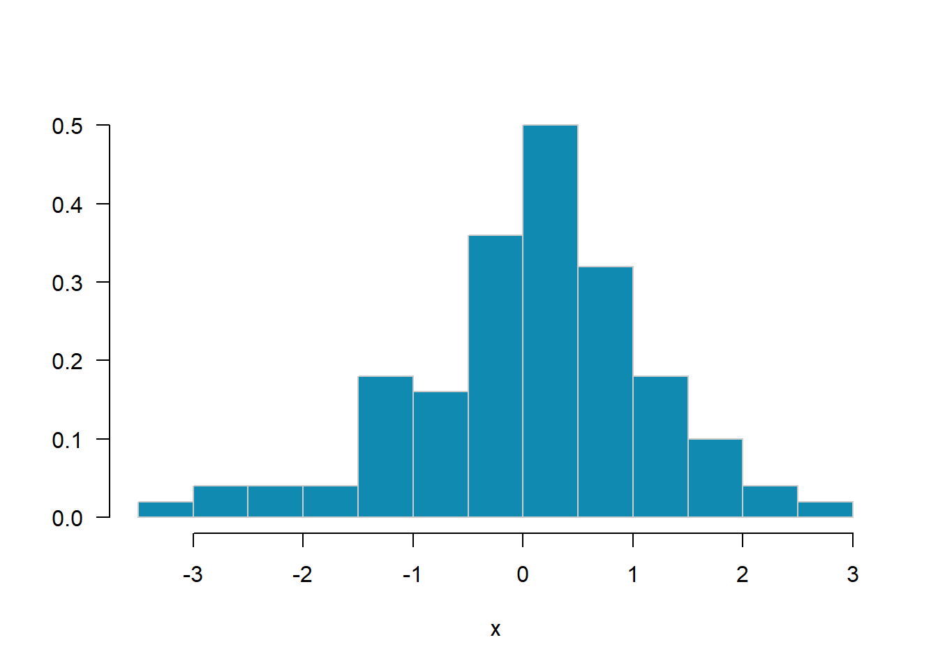
Generate a random sample \(x_1, \ldots, x_{100}\) of data from the \(t_4\) (df=4) distribution using the rt function. Use the MASS::truehist function to display a probability histogram of the sample.

set.seed(1234)
x <- rt(n=100, df=4)
MASS::truehist(x, las=1, col="#118ab2", border="grey80", nbins=20)

Q1.2

Add the \(t_4\) density curve (dt) to your histogram in Exercise 1.1 using the curve function with add=TRUE.

MASS::truehist(x, las=1, col="#118ab2", border="grey80", nbins=20)
curve(dt(x, df=4), from=-4, to=4, add=T, type="l")

Q1.3

Add an estimated density curve to your histogram in Exercise 1.2 using density.

MASS::truehist(x, las=1, col="#118ab2", border="grey80", nbins=20)
curve(dt(x, df=4), from=-4, to=4, add=T, type="l")
lines(density(x), col="firebrick", lwd=2)

Q1.4a

Write an R function f in R to implement the function \(f(x) = (x-a)/b\) that will transform an input vector \(x\) and return the result. The function should take three input arguments: x, a, and b.

f <- function(x, a, b) (x-a)/b

Q1.4b

To transform \(x\) to the interval \([0,1]\) we subtract the minimum value and divide by the range: y <- f(x, a=min(x), b=max(x)-min(x)). Generate a random sample of a Normal(\(\mu=2\), \(\sigma=2\)) data using rnorm and use your function f to transform this sample to the interval \([0,1]\). Print a summary of both the sample x and the transformed sample y to check the result.

set.seed(1234)
x <- rnorm(100, mean=2, sd=2)
y <- f(x, min(x), max(x)-min(x))
data.frame(x=x, y=y) |> summary()

       x                 y         
 Min.   :-2.6914   Min.   :0.0000  
 1st Qu.: 0.2093   1st Qu.:0.2963  
 Median : 1.2307   Median :0.4007  
 Mean   : 1.6865   Mean   :0.4472  
 3rd Qu.: 2.9424   3rd Qu.:0.5755  
 Max.   : 7.0980   Max.   :1.0000  

Q1.5

Refer to Exercise 1.4. Suppose that we want to transform the x sample so that it has mean zero and standard deviation one (studentize the sample). That is, we want \(z_i = (x_i-\bar{x})/s\) for \(i=1,\ldots,n\), where \(s\) is that standard deviation of the sample. Using your function f this is z <- f(x, a=mean(x), b=sd(x)). Display a summary and histogram of the studentized sample z. It should be centered exactly at zero. Use sd(z) to check that the studentized sample has standard deviation exactly 1.0.

z <- f(x, a=mean(x), b=sd(x))
c(mean=mean(z), sd=sd(z)) |> round(10)

mean   sd 
   0    1 

Q1.6

Using your function f of Exercise 1.4, center and scale your Normal(\(\mu=2\), \(\sigma=2\)) sample by subtracting the sample median and dividing by the sample interquartile range (IQR).

w <- f(x, a=median(x), b=IQR(x))
data.frame(x=x, w=w) |> summary()

       x                 w          
 Min.   :-2.6914   Min.   :-1.4351  
 1st Qu.: 0.2093   1st Qu.:-0.3737  
 Median : 1.2307   Median : 0.0000  
 Mean   : 1.6865   Mean   : 0.1667  
 3rd Qu.: 2.9424   3rd Qu.: 0.6263  
 Max.   : 7.0980   Max.   : 2.1468  

Q1.7

Refer to Example 1.14 where we displayed an array of scatterplots using ggplot with facet_wrap. One of the variables in the mpg data is drv, a characer vector indicating whether the vehicle is front-wheel drive, real-wheel drive, or four-wheel drive. Add color=drv in aes: aes(displ, hwy, color=drv) and display the revised plot. Your scatterplots should now have automatically generated a legend for drv color.

library(ggplot2)
mpg |>
    ggplot() + 
    geom_point(aes(displ, hwy, color=drv)) + 
    facet_wrap(~class)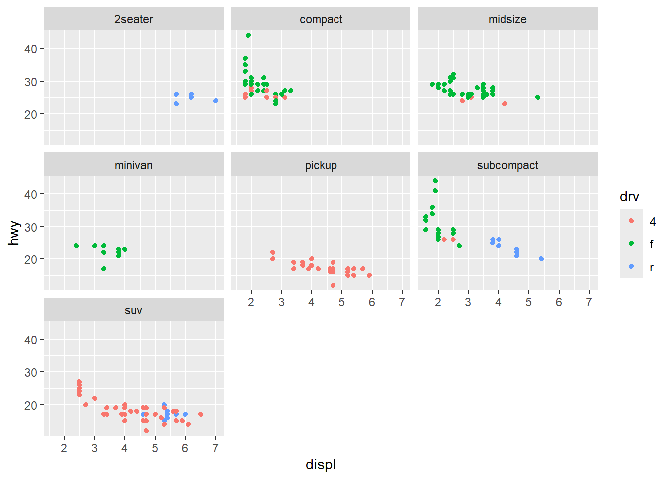

Q1.8

This exercise is intented to serve as an introduction to report writing with R Markdown. Install the knitr package if it is not installed. Create an html report using R Markdown and knitr in RStudio. The report whould include the code and output of Examples 1.12 and 1.14 with appropriate headings and a brief explanation of each example.

Solution Omitted. Note that Quarto supersedes RMarkdown. Visit https://quarto.org/ to learn more.