3  Methods for Generating Random Variables

Q3.1

Write a function that will generate and return a random sample of size \(n\) from the two-parameter exponential distribution Exp(\(\lambda\),\(\eta\)) for arbitrary \(n\), \(\lambda\), and \(\eta\). (See Examples 2.3 and 2.6.) Generate a large sample from Exp(\(\lambda\),\(\eta\)) and compare your sample quantiles with the theoretical quantiles.

Q3.2

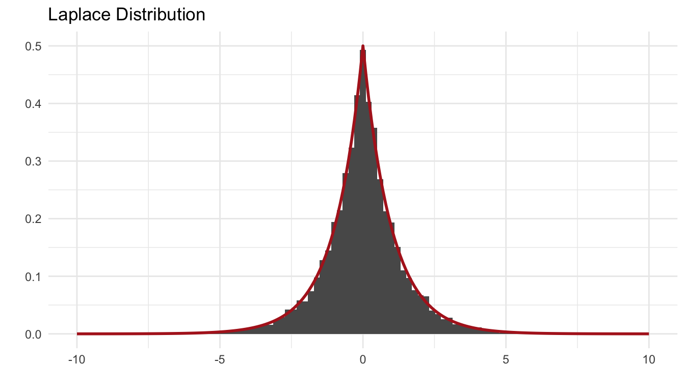
The standard Lapace distribution has density \(f(x) = \frac{1}{2}e^{-\vert x \vert}\) for \(x \in \mathbb{R}\). Use the inverse transform method to generate a random sample of size 1000 from this distribution. Use one of the methods shown in this chapter to compare the generated sample to the target distribution.

Q3.3

The Pareto(\(a\), \(b\)) distribution has cdf

\[ F(x) = 1 - \left(\frac{b}{x}\right)^a, \hspace{1em} x \ge b > 0, \; a > 0 \]

Derive the probability inverse transformation \(F^{-1}(U)\) and use the inverse transform method to simulate a random sample from the Pareto(2,2) distribution. Graph the density histogram of the sample with the Pareto(2,2) density superimposed for comparison.

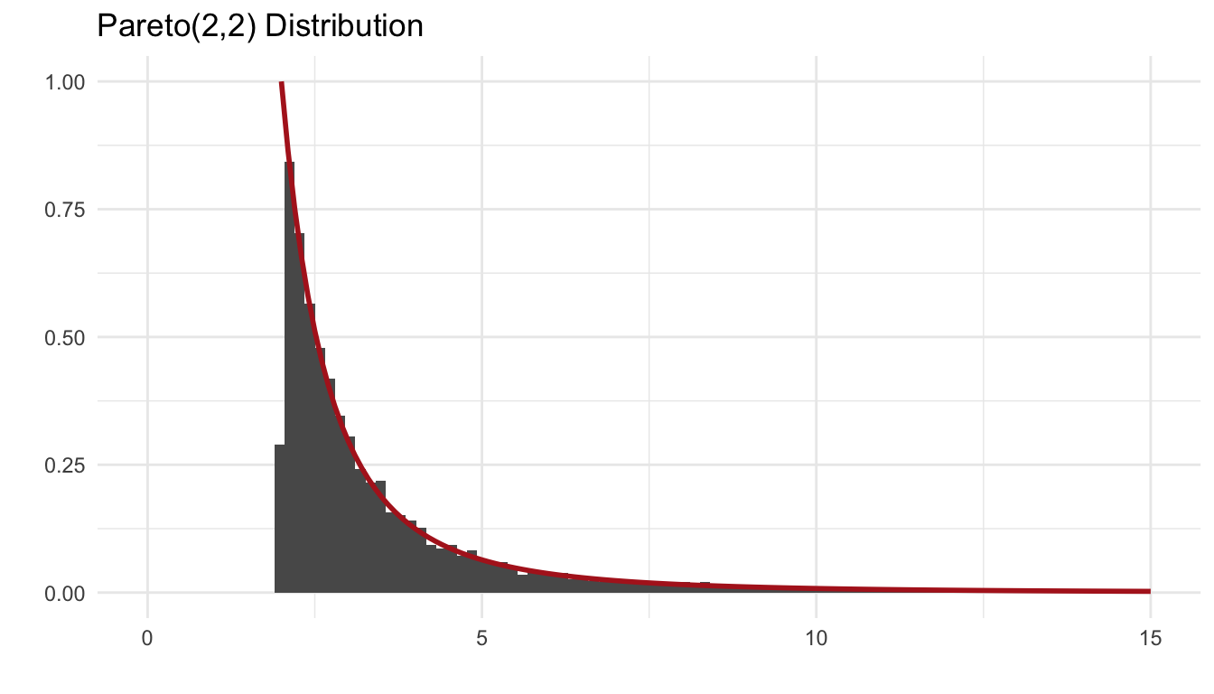
Q3.4

The Rayleigh density is

\[ f(x) = \frac{x}{\sigma^2}e^{-x^2/(2\sigma^2)}, \hspace{1em} x \ge 0, \; \sigma > 0 \]

Develop an algorithm to generate random samples from a Rayleigh(\(\sigma\)) distribution. Generate Rayleigh(\(\sigma\)) samples for several choices of \(\sigma > 0\) and check that the mode of the generated samples is close to the theoretical mode \(\sigma\) (check the histogram).

Q3.5

A discrete random variable \(X\) has probability mass function

[insert table]

Use the inverse transform method to generate a random sample of size 1000 from the distribution of \(X\). Construct a relative frequency table and compare the empirical with the theoretical probabilities. Repeat using the R sample function.

Q3.6

Prove that the accepted variates generated by the acceptance-rejection sampling algorithm are a random sample from the target density \(f_X\).

Q3.7

Write a function to generate a random sample of size \(n\) from the Beta(\(a\), \(b\)) distribution by the acceptance-rejection method. Generate a random sample of size 1000 from the Beta(3,2) distribution. Graph the histogram of the sample with the theoretical Beta(3,2) density superimposed.

Q3.8

Write a function to generate random variates from a Lognormal(\(\mu\), \(\sigma\)) distribution using a transformation method, and generate a random sample of size 1000. Compare the historgram with the lognormal density curve given by the dlnorm function in R.

Q3.9

The rescaled Epanechnikov kernal is a symmetric density function

\[ f_e{x} = \frac{3}{4}(1-x^2), \hspace{1em} \vert x \vert \le 1 \]

Devroye and Gyorfi give the following algorithm for simulation from this distribution. Generate iid \(U_1, U_2, U_3 \sim \text{Uniform}(-1,1)\). If \(\vert U_3 \vert \ge \vert U_2 \vert\) and \(\vert U_3 \vert \ge \vert U_1 \vert\), deliver \(U_2\); otherwise deliver \(U_3\). Write a function to generate random variates from \(f_e\), and construct the histrogram density estimate of a large simulated random sample.

Q3.10

Prove that the algorithm given in Exercise 3.9 generates variates from the density \(f_e\).

Q3.11

Generate a random sample of size 1000 from a normal location mixture. The components of the mixture have \(N(0,1)\) and \(N(3,1)\) distributions with mixing probabilities \(p_1\) and \(p_2 = 1 - p_1\). Graph the histogram of the sample with density superimposed, for \(p_1 = 0.75\). Repeat with different values for \(p_1\) and observe whether the empirical distribution of the mixture appears to be bimodal. Make a conjecture about the values of \(p_1\) that produce bimodal mixtures.

Q3.12

Simulate a continuous Exponential-Gamma mixture. Suppose that the rate parameter \(\Lambda\) has Gamma(\(r\), \(\beta\)) distribution and \(Y\) has Exp(\(\Lambda\)) distribution. That is, \((Y \vert \Lambda = \lambda) \sim f_Y(y \vert \lambda) = \lambda e^{-\lambda y}\). Generate 1000 random observations from this mixture with \(r=4\) and \(\beta=2\)

Q3.13

It can be shown that the mixture in Exercise 3.12 has a Pareto distibution with cdf

\[ F(y) = 1 - \left( \frac{\beta}{\beta + y} \right)^r, \hspace{1em} y \ge 0\]

(This is an alternative parameterization of the Paredo cdf given in Exercise 3.3.) Generate 1000 random observations from the mixture with \(r=4\) and \(\beta = 2\). Compare the empirical and theoretical (Pareto) distributions by graphing the density histogram of the sample and superimposing the Pareto density curve.

Q3.14

Generate 200 random observations from the 3-dimensional multivariate normal distribution having mean vecter \(\mu = (0,1,2)\) and covariance matrix

\[ \Sigma = \begin{bmatrix} 1.0 & -0.5 & 0.5 \\ -0.5 & 1.0 & -0.5 \\ 0.5 & -0.5 & 1.0 \end{bmatrix} \]

using the Choleski factorization method. Use the R pairs plot to graph an arrach of scatter plots for each pair of variables. For each pair of variables (visually) check that the location and correlation approximately agree with the theoretical parameters of the correponding bivariate normal distribution.

Q3.15

Write a function that will standardize a multivariate normal sample for arbitrary \(n\) and \(d\). That is, transform the sample so that the sample mean vector is zero and sample covariance is the identity matrix. To check your results, generate multivariate normal samples and print the sample mean vector and covariance matrix before and after standardization.

Q3.16

Efron and Tibshirani discuss the scor (bootstrap) test score data on 88 students who took examizations in five subjects. Each row of the data frame is a set of scores \((x_{i1}, \ldots, x_{i5})\) for the \(i^{th}\) student. Standardize the scores by type of exam. That is, standardize the bivariate samples (\(X_1, X_2\)) (closed book) and the trivariate samples (\(X_3, X_4, X_5\)) (open book). Compute the covariance matrix of the transformed sample of test scores.

Q3.17

Compare the performance of the Beta generator of Exercise 3.7, Example 3.8, and the R generator rbeta. Fix the parameters \(a=2\), \(b=2\) and time each generator of 1000 iterations with sample size 5000. (See Example 3.19.) Are the results different for different choices of \(a\) and \(b\)?

Q3.18

Write a function to generate a random sample from a \(W_d(\Sigma,n)\) (Wishart) distribution for \(n > d+1 \ge 1\), based on Bartlett’s decomposition.